The Concept of GPU Compiler
Basically, a CPU is a SISD (Single Instruction Single Data) architecture in each core. The multimedia instructions in CPUs are smaller-scale forms of SIMD (Single Instruction Multiple Data), while GPUs are large-scale SIMD processors, capable of coloring millions of image pixels in just a few milliseconds.
Since 2D and 3D graphic processing offers great potential for parallel data processing, GPU hardware typically includes tens of thousands of functional units per chip, as seen in products by NVIDIA and other manufacturers.
This chapter provides an overview of how 3D animation is created and executed on a CPU+GPU system. Following that, it introduces GPU compilers and hardware features relevant to graphics applications. Finally, it explains how GPUs have taken on more computational tasks traditionally handled by CPUs, through the GPGPU (General-Purpose computing on Graphics Processing Units) concept and the emergence of related standards.
Website: Basic Theory of 3D Graphics with OpenGL [1].
Concept in Graphics and Systems
3D Modeling
By creating 3D models with triangles or quads on a surface, the model is formed using a polygon mesh [2]. This mesh consists of all the vertices shown in the first image as Fig. 60.
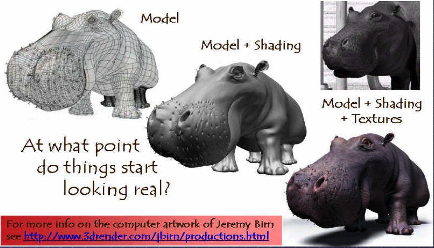
Fig. 60 Creating 3D model and texturing
After applying smooth shading [2], the vertices and edge lines are covered with color (or the edges are visually removed — edges never actually have black outlines). As a result, the model appears much smoother [3].
Furthermore, after texturing (texture mapping), the model looks even more realistic [4].
Animation
★ Animation Layers: High → Low
This breakdown organizes animation systems from the highest gameplay logic down to the lowest GPU skinning, and clearly marks which parts are controlled by the user and which parts are handled by the 3D engine.
Gameplay Animation Logic (High Level): set by user (game developer)
See video here [5].
Examples
Play “walk” when speed > 0.1
Trigger “jump” on button press
Switch to “attack” when enemy detected
Blend run when velocity increases
Where it lives
Live in gameplay scripts (C#, Blueprints, GDScript, Python)
Unity: C# scripts
Unreal: Blueprints or C++
Godot: GDScript
ThinMatrix: Java (no scripting layer)
This layer decides when animations should play.
Animation State Machine / Animation Graph: set by user (game developer)
Examples
Idle → Walk → Run transitions
Blend trees
Animation layers (upper body, lower body)
Animation parameters (speed, grounded, direction)
Where it lives
Unity: Animator Controller
Unreal: Animation Blueprint
Godot: AnimationTree
ThinMatrix: Does not have this layer
This layer controls which animation clip is active and how transitions occur.
Animation Clip Playback Layer: user chooses
An animation clip is a sequence of keyframes over a period of time that represents a motion or action.
Examples
Play animation clip
Loop animation
Set animation speed
Crossfade between clips
Blend two clips together
Who sets it? User chooses which clip to play.
Who implements it? Engine handles blending, timing, and playback.
Where it lives
Unity: Mecanim runtime
Unreal: AnimInstance
Godot: AnimationPlayer
ThinMatrix: Java engine code (Animator.java)
This layer executes the user’s choices.
Skeleton Animation System (Low Level): 3D engine implements it
Examples
Bone hierarchy
Keyframe interpolation
Joint transforms
Matrix palette generation
Pose calculation
Who sets it? Engine
Who uses it? User indirectly, by playing animations.
Where it lives
Unity: C++ engine core
Unreal: C++ engine core
Godot: C++ engine core
ThinMatrix: Java engine code (he writes this manually)
This layer performs the mathematical work of animation.
GPU Skinning (Lowest Level): 3D engine implements it
Examples
Vertex shader skinning
Applying bone matrices
Weighted vertex deformation
Sending matrices to GPU
Who sets it? Engine
Who uses it? User never touches this layer directly (except in custom engines).
Where it lives
Unity: C++ + HLSL
Unreal: C++ + HLSL
Godot: C++ + GLSL
ThinMatrix: GLSL shader he writes manually
This is the final stage where the GPU deforms the mesh.
Full Hierarchy (Summary)
HIGH LEVEL (User)
──────────────────────────────────────────────
1. Gameplay Animation Logic
2. Animation State Machine / Animation Graph
3. Animation Clip Playback

LOW LEVEL (Engine)
──────────────────────────────────────────────
4. Skeleton Animation System
5. GPU Skinning
Developers only write the highest‑level animation logic and designed transitions & blends as shown in Fig. 61. The engine automatically handles all lower‑level animation work. Like the video [5], Jason’s tutorials operate only in Level 1 and Level 2:
✔ Level 1 — Scripts
He writes code like:
animator.SetFloat("Speed", speed);
✔ Level 2 — State Machine
He configures transitions and parameters.
![digraph AnimationLayers {
rankdir=TB;
node [shape=box, style=rounded, fontsize=12];
High1 [label="1. Gameplay Animation Logic\n(User scripts / gameplay code)"];
High2 [label="2. Animation State Machine / Animation Graph\n(User-designed transitions & blends)"];
Mid [label="3. Animation Clip Playback\n(Engine-controlled timing & blending)"];
Low1 [label="4. Skeleton Animation System\n(Bone transforms, keyframe interpolation)"];
Low2 [label="5. GPU Skinning\n(Vertex shader applies bone matrices)"];
High1 -> High2 [label="animation intent\n(e.g., walk, run, jump)"];
High2 -> Mid [label="selected clip + blend parameters"];
Mid -> Low1 [label="sampled pose\n(bone transforms per frame)"];
Low1 -> Low2 [label="matrix palette\n(bone matrices sent to GPU)"];
}](_images/graphviz-d5aaecd7d1d38ca7ea793a9abfc39f0c4b548ed0.png)
Fig. 61 Animation levels
ThinMatrix’s engine collapses the top three layers into Java because it has no scripting layer and no animation graph, so the user must modify the engine code directly.
According to the video on ThinMatrix’s skeleton animation [6], he is sampling the animation clip at different times. The animation clip already contains: keyframes, bone transforms, timestamps, interpolation curves. All of this comes from Blender’s exported .dae file. Joints are positioned at different poses at specific times (keyframes), as illustrated in Fig. 62.
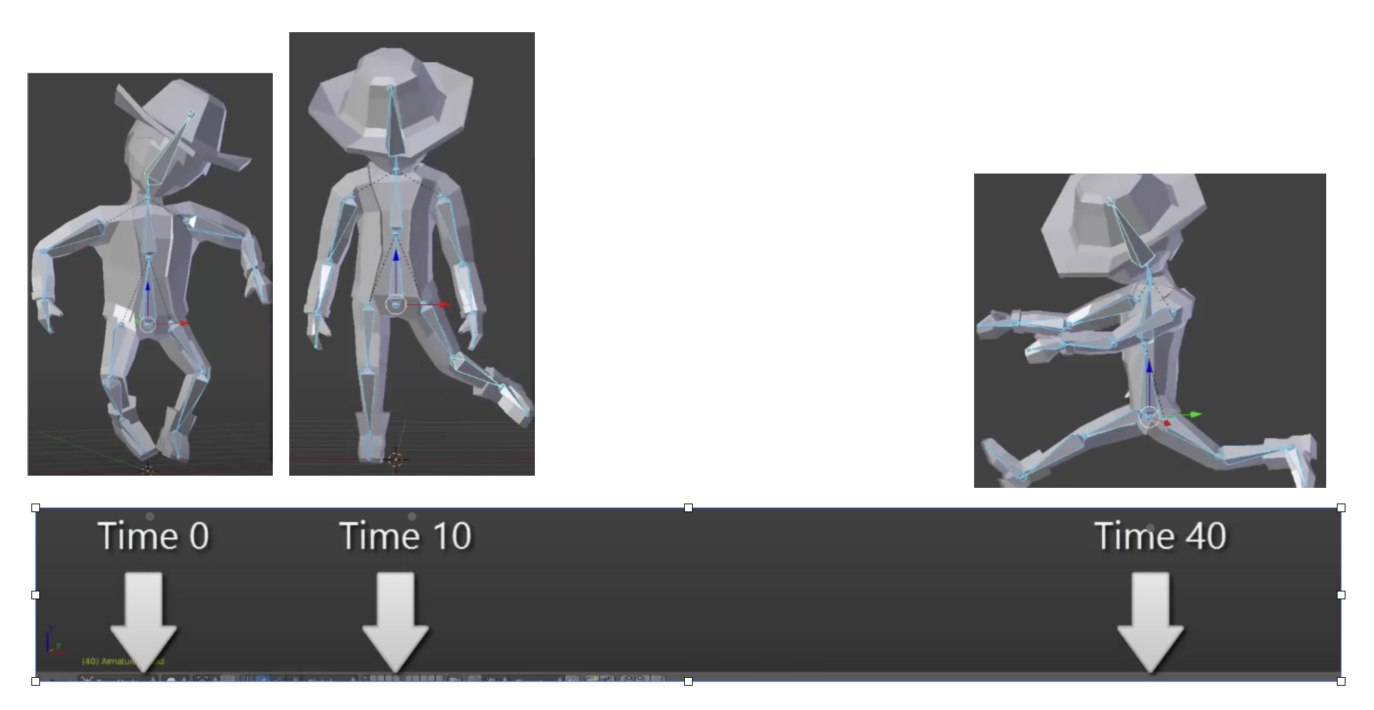
Fig. 62 Get time points at keyframes
Although most of 3D game engines are written C++, ThinMatrix’s engine is 100% Java. In this series of videos, you will see that he writes new Java engine modules, edits existing engine code, loads animation data from Blender, interpolates keyframes, updates bone matrices and sends them to the GPU. Because ThinMatrix’s engine is tiny and educational for engine programmer or game developer, does not provide Scripting Layer (such as C#, Python, GDScript, Blueprints) most commercial 3D engines. Instead, he modifies ThinMatrix’s Java engine directly, which differs from most other 3D engines operate.
Animation flow
Every modern 3D animation tool comes with its own built‑in render engine, and often more than one. In 3D game design, game engines (Unity, Unreal, Godot) use real‑time engines for real-time animation.
Pipeline: Blender → Engine → OpenGL
+------------------+
|     Blender      |
|  (Modeling Tool) |
+------------------+
          |
          |  Exports assets:
          |  - Meshes (.obj, .fbx, .gltf)
          |  - Armatures / bones
          |  - Animations (keyframes)
          |  - Textures (PNG, EXR, TGA)
          v
+---------------------------+
|       Game Engine         |
| (Unity, Unreal, Godot,    |
|  LWJGL, JOGL, Custom)     |
+---------------------------+
          |
          |  Engine loads assets:
          |  - Parses mesh data
          |  - Loads skeletons
          |  - Loads animation curves
          |  - Loads materials/shaders
          |
          |  Engine code you write:
          |  - Java (JOGL/LWJGL)
          |  - C++ (custom engine)
          |  - C# (Unity)
          |  - GDScript/C++ (Godot)
          |
          |  Engine compiles shaders:
          |  - GLSL (OpenGL)
          |  - HLSL (DirectX)
          |  - SPIR-V (Vulkan)
          v
+---------------------------+
|         Renderer          |
|    (OpenGL / Vulkan /     |
|     DirectX / Metal)      |
+---------------------------+
          |
          |  GPU receives:
          |  - Vertex buffers
          |  - Index buffers
          |  - Textures
          |  - Uniforms (matrices, bones)
          |  - Compiled shaders
          v
+---------------------------+
|            GPU            |
| (Vertex Shader → Raster → |
|  Fragment Shader → Frame) |
+---------------------------+
          |
          v
+---------------------------+
|        Final Image        |
|     (On your screen)      |
+---------------------------+
Note
- 3D modeling tools do store animation and movement data
— but they do NOT store any rendering or API‑specific code.
- Game engines do store animation data
— but programmers still write the logic that plays, blends, and controls those animations.
Animation Data vs. Movement Speed in Games
List the animation types in a table for inclusion in this book.
Animation Type |
What Moves |
Description |
GPU Requirement |
|---|---|---|---|
Transform Animation |
Object transform |
The entire mesh moves as a rigid body using position, rotation, and scale. No vertex-level deformation occurs. |
Optional (fixed-function or shaders) |
Skinning |
Vertex positions |
Vertices are blended by bone matrices to deform the mesh (arms bending, legs walking). Requires per-vertex matrix blending. |
Requires shaders |
Morph Target Animation |
Vertex positions |
Vertices blend between multiple stored shapes (facial expressions, muscle bulges). Uses morph weights to interpolate. |
Requires shaders |
Procedural Deformation |
Vertex positions |
Vertices are modified by mathematical functions (wind, waves, noise, squash-and-stretch). Driven by time or simulation parameters. |
Requires shaders |
Example: Walking Animation: Skinning + Transform Animation
When a character walks in a game, the animation is produced by two different systems working together:
Skinning (Bone Animation) Skinning is responsible for deforming the mesh. It drives the motion of limbs such as legs, arms, spine, and feet. Without skinning, the character would move as a rigid statue with no bending or articulation.
Transform Animation (Rigid-Body Movement) Transform animation moves the entire character through the world. This includes translation, rotation, and root motion. Without transform animation, the character would walk in place without actually moving forward.
Root bone: the bone that represents the entire object’s transform — the top‑most parent of the hierarchy. An example of person:
Root
 └─ Pelvis
     ├─ Spine
     │   ├─ Chest
     │   │   ├─ Neck
     │   │   │   └─ Head
     │   │   └─ Shoulders
     │   │       ├─ Arm_L
     │   │       └─ Arm_R
     ├─ Leg_L
     └─ Leg_R
Both systems are required to create a complete walking animation:
Skinning provides the internal limb motion.
Transform animation provides the external world-space movement.
Together, they produce the final effect of a character walking naturally through the environment.
The following explains what animation data 3D modeling tools store, what game engines store, and what programmers must implement manually. It also clarifies the relationship between animation curves, movement speed, and gameplay logic.
What 3D Modeling Tools Actually Store
3D modeling and animation tools such as Blender, Maya, and 3ds Max store animation data, not gameplay logic.
They do store:
Keyframes (frame 0, frame 10, frame 24, etc.)
Bone transforms at each keyframe
Interpolation curves (Bezier, linear, quaternion)
Animation duration (e.g., 1.2 seconds)
Frame rate (e.g., 24 fps)
Skeleton hierarchy
Skin weights (vertex-to-bone influences)
Optional root bone motion (displacement over time)
Modeling tools produce data, not rendering code and not gameplay rules in OpenGL/DirectX code.
Example:
Bone "Arm" rotation at frame 0 = (0°, 0°, 0°)
Bone "Arm" rotation at frame 10 = (45°, 0°, 0°)
What Game Engines Actually Store
The engine’s built‑in C++ renderer handles all OpenGL/Vulkan/Metal calls automatically. Game engines such as Unity, Unreal Engine, Godot, or custom engines store and manage animation data, but still do not define gameplay movement speed.
They do store:
Animation clips
State machines (Idle → Walk → Run)
Blend trees
Transition rules
Animation events
Curves for rotation, scaling, and root motion
Again: data, not OpenGL/DirectX code.
Example:
If speed < 0.1 → Idle
If speed > 0.1 → Walk
If speed > 4.0 → Run
This is engine logic, not GPU code.
Game engines interpret animation data but rely on programmer logic to control how characters move in the world.
What Programmers Must Implement
Programmers write the logic that uses animation data to move objects.
Examples:
In Unity (C#)
animator.SetFloat("speed", playerVelocity);
...
float speed = 3.5f;
transform.position += direction * speed * Time.deltaTime;
In a custom engine (C++/OpenGL)
shader.setMatrix("boneMatrices[0]", boneMatrix);
...
float velocity = 3.5f;
position += velocity * deltaTime;
In JOGL/LWJGL (Java)
glUniformMatrix4fv(boneLocation, false, boneMatrixBuffer);
...
float velocity = 3.5f;
position += velocity * deltaTime;
Programmers write:
Programmers implement:
Movement speed
E.g. Set the value for speed or velocity as the code above.
Acceleration and deceleration
Physics integration
AI movement
Player input
Animation blending logic
Uploading bone matrices to the GPU
GLSL shader code for skinning
Animation data is used by code, not replaced by it.
Root Motion vs. Movement Speed
Some animations include root motion, where the root bone moves forward during a walk cycle. Modeling tools export this as bone displacement over time, but they still do not define speed.
Example:
If the root bone moves 1 meter in 0.5 seconds, the engine can compute:
speed = 1m / 0.5s = 2 m/s
However:
Blender does not store “2 m/s”
The engine derives speed from displacement
Programmers decide whether to use root motion or in-place animation
Summary Table
Concept |
Stored in Blender? |
Stored in Engine? |
Controlled by Programmer? |
|---|---|---|---|
Keyframes |
Yes |
Yes |
No |
Bone transforms |
Yes |
Yes |
No |
Animation length |
Yes |
Yes |
No |
Movement speed |
No |
Yes (derived) |
Yes |
Physics movement |
No |
Yes |
Yes |
AI movement |
No |
Yes |
Yes |
Final Clarification
3D modeling tools store animation timing, not gameplay speed.
Game engines store animation clips, not movement speed.
Programmers control movement speed, physics, and gameplay behavior.
No tool generates JOGL/OpenGL/Vulkan/DirectX code.
All rendering API calls are written by engine developers or by you in a custom engine.
Example for accelerating playing
Animation Speed vs Engine Rendering (5× Speed)
The following table shows how animation playback, movement speed, and GPU rendering interact when the gameplay speed is multiplied by five. The animation remains 24 fps internally, but its playback time advances five times faster. The GPU continues to render at 60 fps and samples the animation at the current time.
Property |
Original Value |
After 5× Speed |
|---|---|---|
Animation FPS (baked) |
24 fps |
24 fps (unchanged) |
Animation Playback Speed |
1× |
5× |
Steps per Second |
6 steps/sec |
30 steps/sec |
Movement Speed |
6 m/sec |
30 m/sec |
GPU Rendering FPS |
60 fps |
60 fps |
Engine Playing Frames (What GPU Displays) |
Samples animation at 60 fps |
Samples animation at 60 fps (skips/interpolates intermediate animation frames) |
Summary:
The animation does not become 120 fps; it is simply played 5× faster.
The runner appears to take 30 steps per second and move 30 meters per second.
The GPU still renders 60 frames per second.
The engine samples the animation at each rendered frame, so it effectively displays every fifth animation sample, using interpolation for smoothness. For this case, it may display 1 out of 2 animation frames from 3D modeling.
Node-Editor (shaders generator)
3D animation tools (Blender, Maya, Houdini) use render engines and node editors for materials, lighting, and effects.
Game engines (Unity, Unreal, Godot) use real‑time engines and node editors for shaders, VFX, and sometimes logic.
A node editor defines the entire material that is applied to the surface of a 3D object. The shader generated from the node graph runs on every pixel (fragment) of the object’s surface. In this sense, the node editor controls the whole surface, not only a specific region.
However, the node graph can include masks, textures, vertex colors, or procedural patterns that allow the artist to specify which parts of the surface receive a particular effect. These masks do not limit the shader to only part of the surface; instead, they instruct the shader how to behave differently across different regions.
Node-Editor
Example
Let’s say you want:
rust only on the edges
metal everywhere else
In the node editor:
Load a rust texture
Load a metal texture
Use a mask (curvature or hand-painted)
Mix them using a Mix node
The shader still runs on the whole surface, but the mask tells it:
“Use rust here”
“Use metal here”
In summary:
The node editor defines the full material for the entire surface.
Artists can use masks or textures to target specific areas within that surface.
The shader still executes globally, but its output varies based on the mask inputs.
Thus, a node editor controls the whole surface, while masks determine how different parts of that surface are shaded.
For 3D video game engines, the only case where mask data is inside the model file is vertex colors. Everything else lives in textures or material/shader assets.
Procedural Rust on Edges Using Shader Nodes
To demonstrate how to create a rust-on-edges material using Blender’s shader node editor as shown in Fig. 63. The goal is to reproduce the effect commonly used on metal containers: clean metal on flat surfaces and rust accumulation along exposed edges.
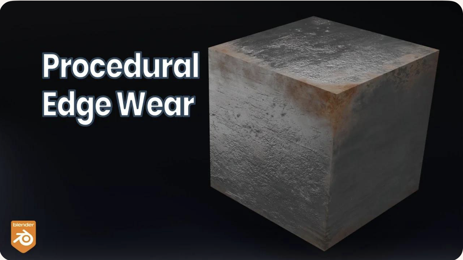
Fig. 63 An example to Rust on Edges Using Shader Nodes [8].
The technique relies on three core ideas:
Detecting edges using the Bevel or Pointiness attribute.
Creating a mask that isolates only the worn edges.
Blending a rust material with a metal material using that mask.
This workflow is fully procedural and does not require painting or external textures.
Procedural Edge Wear Node Graph (ASCII Diagram) to create Fig. 63 in video [8] includes 1. edge detection, 2. mask breakup, 3. material creation, and 4. final blending as follows:
+================================================================+
|                    1.  EDGE DETECTION BLOCK                    |
|                     (Generating an Edge-Wear Mask)             |
+================================================================+

   Geometry Node
        |
        |----> Pointiness (Cycles only)
        |
   Bevel Node (Eevee/Cycles)
        Radius = 0.01–0.03
        |
        v
   ColorRamp (Sharpen edge highlight)
        |
        v
   Edge Mask (base convex-edge detection)


+================================================================+
|              2. MASK BREAKUP / RANDOMIZATION BLOCK             |
|               (Refining the Mask With Noise Textures)          |
+================================================================+

   Noise Texture (Scale 5–15)
        |
        v
   ColorRamp (optional shaping)
        |
        v
   Multiply Node  <---------------- Edge Mask
        |
        v
   ColorRamp (final threshold control)
        |
        v
   Final Edge Wear Mask

material creation
+================================================================+
|                      3. MATERIAL BLOCK                         |
|                       (Base Material Structure)                |
+================================================================+

   METAL MATERIAL:
        Principled BSDF
        Metallic = 1.0
        Roughness = 0.2–0.4

   RUST MATERIAL:
        Principled BSDF
        Base Color = orange/brown
        Roughness = 0.7–1.0
        Optional Noise → color variation
        Optional Bump → rust height


+================================================================+
|                      4. BLENDING BLOCK                         |
|                       (Blending Metal and Rust Materials)      |
+================================================================+

   Metal BSDF ----------------------+
                                    |
                                    v
                               Mix Shader ----> Material Output
                                    ^
                                    |
   Rust BSDF -----------------------+
                                    |
                                    |
                         Final Edge Wear Mask (Fac)
Code Generation from Node-Editor
Node-based shader editors are visual tools used in modern game engines and DCC (Digital Content Creation) software. They allow users to build shaders by connecting nodes instead of writing GLSL, HLSL, or Metal code manually. These editors do generate shader code automatically.
Node-Based Editors Do Generate Shader Code
Node-based shader editors such as:
Unity Shader Graph
Unreal Engine Material Editor
Godot Visual Shader Editor
Blender Shader Nodes (for Eevee/Cycles)
all compile the visual node graph into real shader code.
Depending on the engine, the generated code may be:
GLSL (OpenGL / Vulkan)
HLSL (DirectX)
MSL (Metal)
SPIR-V (Vulkan intermediate format)
The generated code is usually not shown to the user, but it is compiled and sent to the GPU at runtime.
How Users Generate Shader Code with Nodes
The workflow for generating shader code through a node editor typically looks like this:
The user opens the shader editor.
The user creates nodes representing:
math operations (add, multiply, dot product)
texture sampling
Determine FS.
lighting functions
color adjustments
UV transformations
The user connects nodes visually to define the shader logic.
Defines surface color,lighting, and texture sampling → determine FS.
For simple deformations (waves, wind, dissolve) → determine the VS.
Generate both TCS and TES code for displacement and subdivision control.
GS code is typically written manually by graphics programmers since primitives culling and clipping are not related with model resolution and texture materials.
The engine converts the node graph into an internal shader representation.
The engine compiles this representation into platform-specific shader code (GLSL, HLSL, MSL, or SPIR-V).
The compiled shader is sent to the GPU and used for rendering.
The user never writes the shader code directly; the editor generates it automatically.
Who Is the “User” of Node-Based Editors?
The typical users of node-based shader editors are:
- Graphics Designers / Technical Artists
Primary users.
They create visual effects, materials, and surface shaders.
They usually do not write GLSL or HLSL manually.
Node editors allow them to work visually without programming.
- Software Programmers / Graphics Programmers
Secondary users.
They may create custom nodes or extend the shader system.
They write low-level shader code when needed.
They integrate the generated shaders into the rendering pipeline.
In most workflows:
Graphics designers build the shader visually.
The engine generates the shader code.
Programmers handle advanced logic, optimization, or custom nodes.
Summary
Node-based shader editors do generate shader code automatically.
Users generate shaders by connecting visual nodes rather than writing GLSL/HLSL manually.
The primary “user” is the graphics designer or technical artist.
Programmers support the system by writing custom nodes or low-level shaders when needed.
The shaders introduction is illustrated in the next section OpenGL.
3D Modeling Tools
Every CAD software manufacturer, such as AutoDesk and Blender, has their own proprietary format. To solve interoperability problems, neutral or open source formats were created as intermediate formats to convert between proprietary formats.
Naturally, these neutral formats have become very popular. Two famous examples are STL (with a .STL extension) and COLLADA (with a .DAE extension). Below is a list showing 3D file formats along with their types.
3D file format |
Type |
|---|---|
STL |
Neutral |
OBJ |
ASCII variant is neutral, binary variant is proprietary |
FBX |
Proprietary |
COLLADA |
Neutral |
3DS |
Proprietary |
IGES |
Neutral |
STEP |
Neutral |
VRML/X3D |
Neutral |
The four key features a 3D file can store include the model’s geometry, the model’s surface texture, scene details, and animation of the model [9].
Specifically, they can store details about four key features of a 3D model, though it’s worth bearing in mind that you may not always take advantage of all four features in all projects, and not all file formats support all four features!
3D printer applications do not to support animation. CAD and CAM such as designing airplane does not need feature of scene details.
DAE (Collada) appeared in the video animation above. Collada files belong to a neutral format used heavily in the video game and film industries. It’s managed by the non-profit technology consortium, the Khronos Group.
The file extension for the Collada format is .dae. The Collada format stores data using the XML mark-up language.
The original intention behind the Collada format was to become a standard among 3D file formats. Indeed, in 2013, it was adopted by ISO as a publicly available specification, ISO/PAS 17506. As a result, many 3D modeling programs support the Collada format.
That said, the consensus is that the Collada format hasn’t kept up with the times. It was once used heavily as an interchange format for Autodesk Max/Maya in film production, but the industry has now shifted more towards OBJ, FBX, and Alembic [9].
Graphics HW and SW Stack
This section provides a more detailed illustration of animation accross the software and hardware stacks on both CPU and GPU, and explains how data flows between the CPU, the GPU, and each layer of the software stack.
In the previous section 3D Modeling, described what information 3D models store and how this information is used to perform animation.
In the incoming section SW Stack and Data Flow will describe how each frame is generated to display the movement animation or skinning effects using the small animation parameters stored in 3D model and sent from CPU.
The the incoming section Role and Purpose of Shaders will explain different visual effects can be achieved by switching shaders to shapplying different materials across frames.
Reference:
HW Block Diagram
The block diagram of the Graphic Processing Unit (GPU) is shown in Fig. 64.
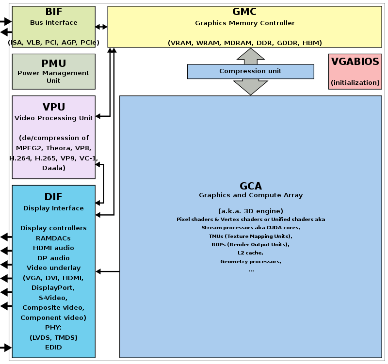
Fig. 64 Components of a GPU: GPU has accelerated video decoding and encoding [10]
The roles of the CPU and GPU in graphic animation are illustrated in Fig. 65.
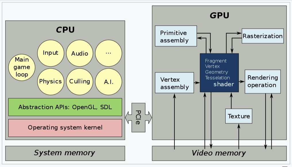
Fig. 65 OpenGL and Vulkan are both rendering APIs. In both cases, the GPU executes shaders, while the CPU executes everything else [11].
GPU can’t directly read user input from, say, keyboard, mouse, gamepad, or play audio, or load files from a hard drive, or anything like that. In this situation, cannot let GPU handle the animation work [12].
A graphics driver consists of an implementation of the OpenGL state machine and a compilation stack to compile the shaders into the GPU’s machine language. This compilation, as well as pretty much anything else, is executed on the CPU, then the compiled shaders are sent to the GPU and are executed by it. (SDL = Simple DirectMedia Layer) [13].
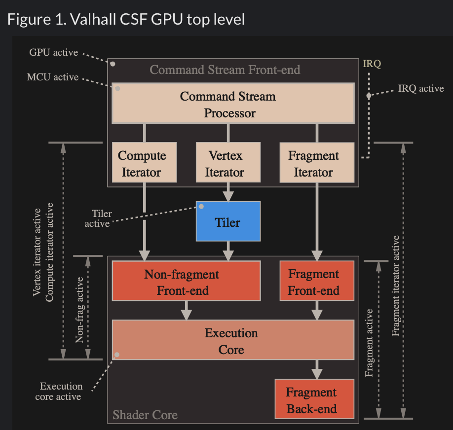
Fig. 66 MCU and specific HW circuits to speedup the processing of CSF (Command Stream Fronted) [14].
The GPU driver write command and data from CPU to GPU’s system memory through PCIe. These commands are called Command Stream Fronted (CSF) in the memory of GPU. A chipset of GPU includes tens of SIMD processors (cores). In order to speedup the GPU driver’s processing, the CSF is designed to a simpler form. As result, GPU chipset include MCU (Micro Chip Unit) and specfic HW to transfer the CSF into individual data structure for each SIMD processor to execute as Fig. 66. The firmware version of MCU is updated by MCU itself usually.
SW Stack and Data Flow
The driver runs on the CPU side as shown in Fig. 67. The OpenGL API eventually calls the driver’s functions, and the driver executes these functions by issuing commands to the GPU hardware and/or sending data to the GPU.
Even so, the GPU’s rendering work, which uses data such as 3D vertices and colors sent from the CPU and stored in GPU or shared memory, consumes more computing power than the CPU.
![digraph G {
rankdir=LR;
compound=true;
node [shape=record];
subgraph cluster_cpu {
label = "CPU (Client)";
CPU_SW [label=" 3D Model | Game Engine | { OpenGL API | Shaders \n (buitin-functions)} | <f1> Driver"];
}
subgraph cluster_gpu {
label = "GPU HW (Server)";
subgraph cluster_gpu_sw {
label = "3D Rendering pipeline \ndescribed in the later section";
ModelData [label="3D Model Information\n(VAO, VBO, textures,\nindex buffers, materials)"];
}
}
CPU_SW:f1 -> ModelData [label="1. Creating Mesh:\nVAO, texture, ..., from 3D model, \n shader-exectuable-code."];
// label = "Graphic SW Stack";
}](_images/graphviz-d57d5931f1f9ccf5318cd31cb81606a4851808e0.png)
Fig. 67 Graphic SW Stack and data flow in initializing graphic model
✅ As section Animation and Fig. 67. The game engine’s built‑in C++ renderer handles all OpenGL/Vulkan/Metal calls automatically. Users set the value for speed, velocity, …, etc, customize the animation logic.
After the user creates a skeleton and textures for each model and sets keyframe times using a 3D modeling tool, users can write gameplay scripts (Java code, C#, Blueprints, GDScript, Python, etc.) to tell the engine to play animations [7].
As section Node-Editor (shaders generator), the skin materials created by Graphics Designers / Technical Artists and secondly created by Software Programmers / Graphics Programmers using the tool Node-Editor (shaders generator). As result, shaders generated from tool Node-Editor (shaders generator).
Shaders may call built-in functions written in Compute Shaders, SPIR-V, or LLVM-IR. LLVM libclc is a project for OpenCL built-in functions, which can also be used in OpenGL [15]. Like CPU built-ins, new GPU ISAs or architectures must implement their own built-ins or port them from open source projects like libclc.
The 3D model on the CPU performs these animations in movement and others by computing each frame from the stored keyframes, as illustrated in animation section Animation.
![digraph G {
rankdir=LR;
compound=true;
node [shape=record];
subgraph cluster_cpu {
label = "CPU (Client)";
CPU_SW [label=" 3D Model | Game Engine | { OpenGL API | Shaders \n (buitin-functions)} | <f1> Driver"];
}
subgraph cluster_gpu {
label = "GPU HW (Server)";
subgraph cluster_gpu_sw {
label = "3D Rendering pipeline \ndescribed in the later section";
ModelData [label="3D Model Information\n(VAO, VBO, textures,\nindex buffers, materials)"];
UniformUpdates [label="Uniform Updates\n(bone matrices, morph weights,\nmaterial params, time, etc.\nsee Note below)", style=filled, fillcolor=lightgreen, color="black"];
}
}
CPU_SW:f1 -> UniformUpdates [label="2. Animation: \nDraw command and Uniform Updates\nfor each frame rendering"];
// label = "Graphic SW Stack";
}](_images/graphviz-0d075acb82ffbf7b5a9c6454129f2a2adea8b6e4.png)
Fig. 68 Graphic SW Stack and data flow in rendering
The per-frame data is not the full set of vertices, but rather a small set of animation parameters named Uniform Updates as appeared in Fig. 68, which are described later.
Note
Bone matrices determine the positions of triangles within a 3D model during animation. This bone transformation data is much smaller than the complete mesh of the 3D model. We will provide an example and explain this in more detail in the Animation Example section. Because this transformation data is small and constant across all shader pipeline stages, it is stored in the GPU’s global memory and can be cached in the uniform/constant cache for performance, as illustrated in Fig. 123 of Processor Units and Memory Hierarchy in NVIDIA GPU 82 section.
The CPU updates only these small animation parameters and issues draw command to the GPU server side.
![digraph GPU_Pipeline {
rankdir=LR;
node [shape=box, style=rounded, fontsize=12];
UniformUpdates [label="Uniform Updates\n(bone matrices, morph weights,\nmaterial params, time, etc.)"];
ModelData [label="3D Model Information\n(VAO, VBO, textures,\nindex buffers, materials)"];
GPURendering [label="GPU Rendering\n(vertex shader, fragment shader,\nskinning, morphing, rasterization)"];
Framebuffer [label="Framebuffer\n(Video Memory Output)"];
UniformUpdates -> GPURendering;
ModelData -> GPURendering;
GPURendering -> Framebuffer [label="Rendered Image"];
}](_images/graphviz-6d13404837e020997ab2c96aa6f23a40c76dc5e3.png)
Fig. 69 The input and output for GPU rendering
Next, the 3D Rendering-pipeline is illustrated in Fig. 69.
The shape of object data are stored in the form of VAOs (Vertex Array Objects) in OpenGL. This will be explained in a later section OpenGL. Additionally, OpenGL provides VBOs (Vertex Buffer Objects), which allow vertex array data to be stored in high-performance graphics memory on the server side GPU and enable efficient data transfer [16] [17].
After GPU receives the Uniform Updates from CPU, it performs the computationally intensive per‑vertex work within the rendering pipeline to generate the final pixel values for each frame displayed on screen. These final pixel values are collectively referred to the Rendered Image.
✅ “Rendered Image” = the final per‑frame output written into the framebuffer. The Uniform Updates will be described in detail later.
✅ CPU only updates small animation parameters named Uniform Updates as appeared in Fig. 68; GPU computes the heavy per‑vertex work.
As mentioned in the previous section on animation movement, 3D modeling tools store Keyframes, bone transforms at each keyframe and related data, and perform animation based on this information.
The CPU updates only the bone transformation data …, rather than updating the entire vertex or mesh data for each animation frame. These updates are very small—on the order of kilobytes rather than megabytes. For each rendered frame, the CPU sends these small updates to the GPU, and the GPU takes over the animation work from the CPU. This type of movement animation is called skinning, and is illustrated as follows:
Skinning
Skinning is a vertex deformation technique used to animate a mesh by attaching its vertices to a hierarchical skeleton (bones). Each vertex stores one or more bone indices and corresponding weights that describe how strongly each bone influences that vertex.
During animation, the application updates the bone transformation matrices. The vertex shader then computes the final vertex position by blending the transformed positions according to the stored weights. This allows the mesh to bend, twist, and deform smoothly as the skeleton moves.
Skinning does not create new geometry or smooth the surface topology. It only transforms the existing vertices of the mesh. Examples include bending an arm, flapping a wing, or deforming a flexible tube as its bones rotate.
CPU only update high‑level animation state, such as:
Current animation time
Bone matrices (small)
Morph weights
Material parameters
Particle emitter settings
Global uniforms (camera, lights, etc.)
These are tiny updates — kilobytes, not megabytes.
In practice (real engines): the weights are normalized so the sum = 1.0 \(\Rightarrow \sum_{i=0}^{N-1}\mathbf{weight}_i = 1.0\)
Example: Bending an Arm
Imagine a character’s arm mesh. Each vertex in the elbow area has weights like:
70% influenced by upper‑arm bone
30% influenced by lower‑arm bone
When the elbow bends:
Upper‑arm bone rotates
Lower‑arm bone rotates
GPU blends the influence
The elbow area deforms smoothly
This is skinning.
✅ After the GPU animation, the color pixels are write to framebuffer (video memory). The display device (monitor, LCD, OLED, etc.) fetches these pixels and displays them on the screen. The interface between framebuffer and display device is explained in the next section Pixels Displaying.
Pixels Displaying
The interface between frame buffer and displaying device is shown as Fig. 70.
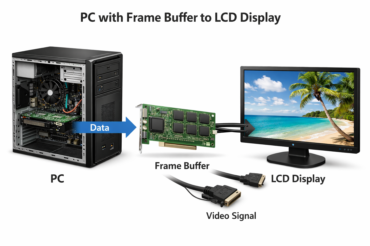
Fig. 70 PC with Frame Buffer to LCD Display
GPU and screen (monitor, LCD, OLED, etc.) use VSync, NVIDIA G-SYNC or AMD FreeSync to prevent screen tearing, as described below:
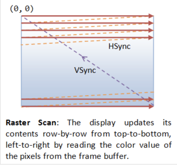
Fig. 71 VSync
VSync
No tearing occurs when the GPU and display operate at the same refresh rate,
since the GPU refreshes faster than the display as shown below.

              A    B

GPU      | ----| ----|

Display  |-----|-----|

            B      A

Tearing occurs when the GPU has exact refresh cycles but VSync takes
one more cycle than the display as shown below.

              A

GPU      | -----|

Display  |-----|-----|

            B      A

To avoid tearing, the GPU runs at half the refresh rate of the display,
as shown below.

              A          B

GPU      | -----|    | -----|

Display  |-----|-----|-----|-----|

            B      B    A     A
Double Buffering
While the display is reading from the frame buffer to display the current frame, we might be updating its contents for the next frame (not necessarily in raster-scan manner). This would result in the so-called tearing, in which the screen shows parts of the old frame and parts of the new frame. This could be resolved by using so-called double buffering. Instead of using a single frame buffer, modern GPU uses two of them: a front buffer and a back buffer. The display reads from the front buffer, while we can write the next frame to the back buffer. When we finish, we signal to GPU to swap the front and back buffer (known as buffer swap or page flip).
VSync
Double buffering alone does not solve the entire problem, as the buffer swap might occur at an inappropriate time, for example, while the display is in the middle of displaying the old frame. This is resolved via the so-called vertical synchronization (or VSync) at the end of the raster-scan. When we signal to the GPU to do a buffer swap, the GPU will wait till the next VSync to perform the actual swap, after the entire current frame is displayed.
As above text digram. The most important point is: When the VSync buffer-swap is enabled, you cannot refresh the display faster than the refresh rate of the display!!! If GPU is capable of producing higher frame rates than the display’s refresh rate, then GPU can use fast rate without tearing. If GPU has same or less frame rates then display’s and you application refreshes at a fixed rate, the resultant refresh rate is likely to be an integral factor of the display’s refresh rate, i.e., 1/2, 1/3, 1/4, etc. Otherwise it will cause tearing [1].
NVIDIA G-SYNC and AMD FreeSync
If your monitor and graphics card both in your customer computer support NVIDIA G-SYNC, you’re in luck. With this technology, a special chip in the display communicates with the graphics card. This lets the monitor vary the refresh rate to match the frame rate of the NVIDIA GTX graphics card, up to the maximum refresh rate of the display. This means that the frames are displayed as soon as they are rendered by the GPU, eliminating screen tearing and reducing stutter for when the frame rate is both higher and lower than the refresh rate of the display. This makes it perfect for situations where the frame rate varies, which happens a lot when gaming. Today, you can even find G-SYNC technology in gaming laptops!
AMD has a similar solution called FreeSync. However, this doesn’t require a proprietary chip in the monitor. In FreeSync, the AMD Radeon driver, and the display firmware handle the communication. Generally, FreeSync monitors are less expensive than their G-SYNC counterparts, but gamers generally prefer G-SYNC over FreeSync as the latter may cause ghosting, where old images leave behind artifacts [18].
The Role and Purpose of Shaders
The flow for 3D/2D graphic processing is shown in Fig. 72.
![digraph G {
rankdir=LR;
compound=true;
node [shape=record];
subgraph cluster_3d {
label = "3D/2D modeling software";
subgraph cluster_code {
label = "3D/2D's code: engine, shader, ...";
Api [label="<a> OpenGL API | <s> Shaders (3D animation's shaders \n or programmer writing shaders"];
}
}
subgraph cluster_driver {
label = "Driver"
Compiler [label="On-line Compiler"];
Obj [label="obj"];
Linker [label="On-line binding (Linker)"];
Exe [label="exe"];
}
Api:a -> Obj [lhead ="cluster_driver"];
Api:s -> Compiler;
Compiler -> Obj -> Linker -> Exe;
Exe -> GPU;
Exe -> CPU [ltail ="cluster_driver"];
// label = "OpenGL Flow";
}](_images/graphviz-9a9d3960428cd44db25d58d9a03d5160f8bb70ca.png)
Fig. 72 OpenGL Flow
The compiled shaders are sent to the GPU when you call glLinkProgram(). That is the moment the driver uploads the compiled shader binaries into GPU‑executable form.
The glLinkProgram() is called when you finish preparing a shader program — not when creating a mesh, and not when issuing a draw command.
When a game actually call glLinkProgram() to re-link the shader, the shader need to be compiled and load to GPU.
Usually it is happend in game startup, level load, or creating a new shader variant (e.g., enabling shadows, fog, skinning).
Games switch shaders constantly — sometimes hundreds of times per frame — but they do not re‑link them.
When playing a video game, different materials, effects and rendering passes will applying to difference shaders.
Examples of switching shaders:
When the player enters a snowy biome, ice meshes use the ice shader.
The axe blade uses a metal PBR shader. Sparks fly when the axe blade hits stone it switch to particle shader.
Basic geometry in computer graphics
This section introduces the fundamental geometry mathematics used in computer graphics. As discussed in the previous sections, 3D animation primarily based on geometric representations such as meshes (vertices) and surface discriptions including textures, materials, shaders, and lighting models created in 3D content creation tools. Consequently, vertex tranformations and lighting-based color computations form the mathematical foundation of modern computer graphics and animation.
The complete concept can be found in the book Computer Graphics: Principles and Practice, 3rd Edition, authored by John F. et al. However, the book contains over a thousand pages.
It is very comprehensive and may take considerable time to understand all the details.
Color
In the case of paints, additive colors produce shades and become light gray due to the addition of darker pigments [21].
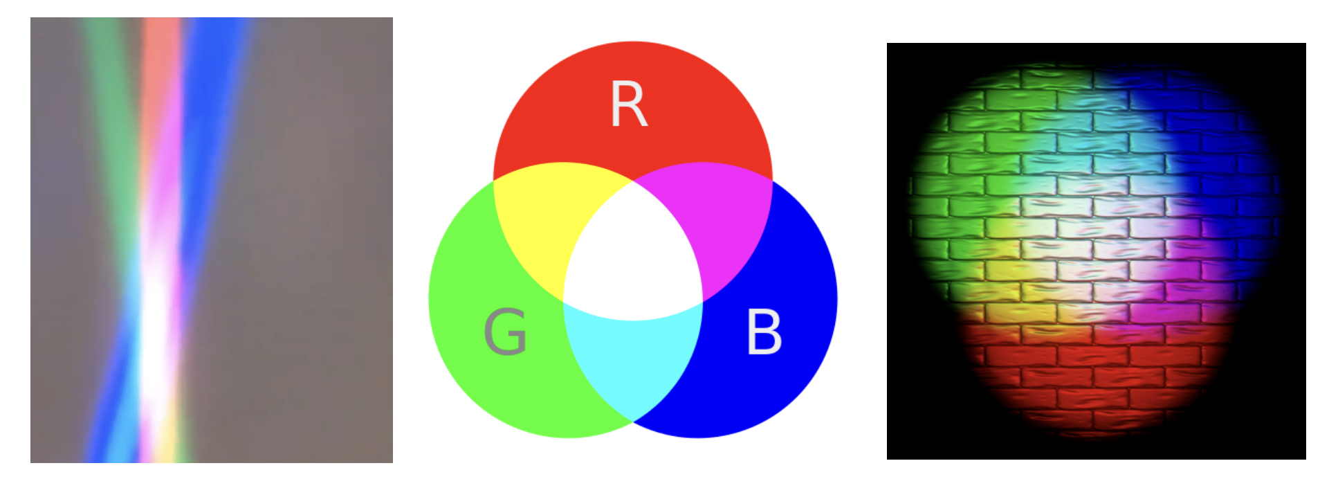
Fig. 73 Additive colors in light
Note
Additive colors
I know it doesn’t match human intuition. However, additive RGB colors in light combine to produce white light, while additive RGB in paints result in light gray paint. This makes sense because light has no shade. This result stems from the way human eyes perceive color. Without light, no color can be sensed by the eyes.
Computer engineers should understand that exploring the underlying reasons falls into the realms of physics or the biology of the human eye structure.
Transformation
Overview
The tranformation matrices have been taught in high school and college. However this mathematical details are not always retained clearly in memory. The following section reviews the parts relevant to graphics rendering.
In both 2D and 3D graphics, every object transformation is performed by multiplying the object’s vertex coordinates by one or more transformation matrices. Modern OpenGL uses homogeneous coordinates and 4×4 matrices to unify translation, rotation, scaling, projection, and even animation (skinning) into a single mathematical framework.
A vertex in 3D is represented as:
A transformation is applied by matrix multiplication:
Multiple transformations are combined by multiplying matrices:
Where:
M= Model matrix (object → world)V= View matrix (world → camera)P= Projection matrix (camera → clip space)
This is the core of the OpenGL rendering pipeline, as shown in Fig. 74.
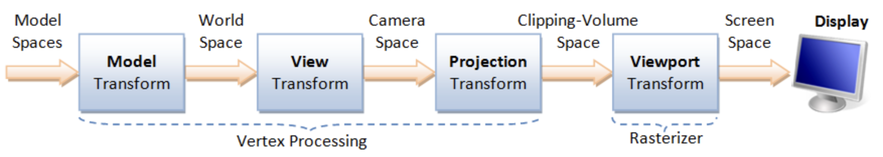
Model space: The is the vertices position mentioned under Root bone in Animation flow. All vertex coordinates are calcuated relative to the root bone.
Model Rranform:
M= Model matrix (object → world). This represents the vertex positions mentioned under Transform Animation in Animation flow.
Details for Fig. 74 can be found on “4. Vertex Processing” of the website [1].
Transformation Matrices [22]
Translation: Moves an object in 3D space.
\(T(x,y,z)=\begin{bmatrix}1&0&0&x\\0&1&0&y\\0&0&1&z\\0&0&0&1\end{bmatrix} \begin{bmatrix}X\\Y\\Z\\1\end{bmatrix} = \begin{bmatrix}X+x\\Y+y\\Z+z\\1\end{bmatrix}\)
Scaling: Resizes an object.
\(S(s_x,s_y,s_z)=\begin{bmatrix}s_x&0&0&0\\0&s_y&0&0\\0&0&s_z&0\\0&0&0&1\end{bmatrix} \begin{bmatrix}X\\Y\\Z\\1\end{bmatrix} = \begin{bmatrix}s_x X\\s_y Y\\s_z Z\\1\end{bmatrix}\)
Rotation X: Rotates around the X-axis.
\(R_x(\theta)=\begin{bmatrix}1&0&0&0\\0&\cos\theta&-\sin\theta&0\\0&\sin\theta&\cos\theta&0\\0&0&0&1\end{bmatrix} \begin{bmatrix}X\\Y\\Z\\1\end{bmatrix} = \begin{bmatrix}X\\Y\cos\theta - Z\sin\theta\\Y\sin\theta + Z\cos\theta\\1\end{bmatrix}\)
Rotation Y: Rotates around the Y-axis.
\(R_y(\theta)=\begin{bmatrix}\cos\theta&0&\sin\theta&0\\0&1&0&0\\-\sin\theta&0&\cos\theta&0\\0&0&0&1\end{bmatrix} \begin{bmatrix}X\\Y\\Z\\1\end{bmatrix} = \begin{bmatrix}X\cos\theta + Z\sin\theta\\Y\\-X\sin\theta + Z\cos\theta\\1\end{bmatrix}\)
Rotation Z: Rotates around the Z-axis.
\(R_z(\theta)=\begin{bmatrix}\cos\theta&-\sin\theta&0&0\\\sin\theta&\cos\theta&0&0\\0&0&1&0\\0&0&0&1\end{bmatrix} \begin{bmatrix}X\\Y\\Z\\1\end{bmatrix} = \begin{bmatrix}X\cos\theta - Y\sin\theta\\X\sin\theta + Y\cos\theta\\Z\\1\end{bmatrix}\)
Shear in X: - Skews geometry along axis X.
\(\text{Shear}_X(a,b)= \begin{bmatrix}1&a&b&0\\0&1&0&0\\0&0&1&0\\0&0&0&1\end{bmatrix} \begin{bmatrix}X\\Y\\Z\\1\end{bmatrix} = \begin{bmatrix}X + aY + bZ\\Y\\Z\\1\end{bmatrix}\)
Shear in Y: Skews geometry along axis Y.
\(\text{Shear}_Y(c,d)= \begin{bmatrix}1&0&0&0\\c&1&d&0\\0&0&1&0\\0&0&0&1\end{bmatrix} \begin{bmatrix}X\\Y\\Z\\1\end{bmatrix} = \begin{bmatrix}X\\cX + Y + dZ\\Z\\1\end{bmatrix}\)
Shear in Z: Skews geometry along axis Z.
\(\text{Shear}_Z(e,f)= \begin{bmatrix}1&0&0&0\\0&1&0&0\\e&f&1&0\\0&0&0&1\end{bmatrix} \begin{bmatrix}X\\Y\\Z\\1\end{bmatrix} = \begin{bmatrix}X\\Y\\eX + fY + Z\\1\end{bmatrix}\)
Reflection: Mirrors across a plane.
\(\text{Reflect}_{XY},\ \text{Reflect}(\mathbf{n})\)
The “4.2 Model Transform (or Local Transform, or World Transform)” of on the website [1] provides conceptual coverage of transformations. List the websites that provide proofs of the non-obvious transformation formulas below.
Rotation
The mathematical proof is given below.
Prove the 2D formula and then intutively extend it to 3D along the X, Y, and Z axes [23].
Proof in greater details:
https://austinmorlan.com/posts/rotation_matrices/
Shear (Skew)
Shear is a skewing transformation as shown in Fig. 75.
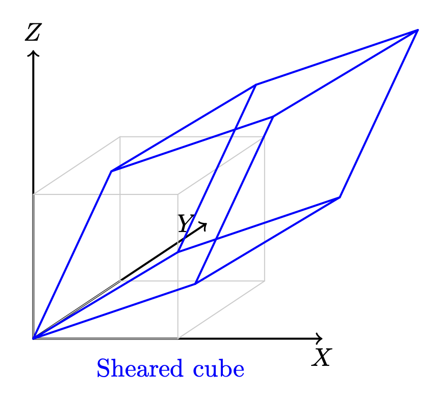
Fig. 75 3D shear
Shear in X: plane x = 0 (the YZ‑plane), slides points parallel to the X‑axis.
The mathematical proof is given below.
https://en.wikipedia.org/wiki/Shear_mapping
Reflection
Reflection is nothing but a mirror image of an object.
Reflection across the XY-plane:
Reflection across an arbitrary plane with unit normal \(\mathbf{n}\):
The mathematical proof is given below.
https://www.geeksforgeeks.org/computer-graphics/computer-graphics-reflection-transformation-in-3d/
The following Quaternion Product (Hamilton product) is from the wiki [24] since it is not covered in the book.
Cross Product
Both triangles and quads are polygons. So, objects can be formed with polygons in both 2D and 3D. The transformation in 2D or 3D is well covered in almost every computer graphics book. This section introduces the most important concept and method for determining inner and outer planes. Then, a point or object can be checked for visibility during 2D or 3D rendering.
Any area of a polygon can be calculated by dividing it into triangles or quads. The area of a triangle or quad can be calculated using the cross product in 3D.
✅ The role of cross product:
In 2D geometry mathematics, \(v_0, v_1 and v_2\) can form the area of a parallelogram as shown in Fig. 76. The fourth vertex, \(\mathbf{v}_3\), can then be determined to complete the parallelogram.
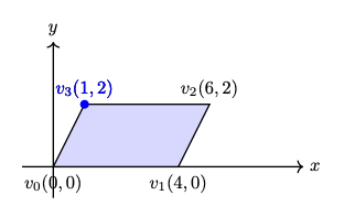
Fig. 76 The area determined by \(v_0, v_1, v_2\) in 2D
The area of the parallelogram is given by:
The area of a parallelogram is same in both 2D and 3D. To extend the definition of the corss product to 3D, all we must additionally consider the orientation of the plane, since a plane has two possible faces.
\(n\) is a unit vector perpendicular to the plane. \(\Rightarrow\) direction.
As shown in Fig. 77, the plane determined by \(v_0, v_1, v_2\) with CCW ordering defines a unique orientation.
The area of the parallelogram remains unchanged after rotation as shown in Fig. 78, which means the area and plane face determined by extending the definition of cross product from 2D to 3D correctly.
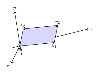
Fig. 77 The area and plane face determined by \(v_0, v_1, v_2\) with CCW ordering before rotation \(z\) axis.¶ |
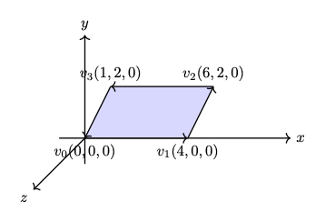
Fig. 78 The area and plane face determined by \(v_0, v_1, v_2\) with CCW ordering after rotation \(z\) axis.¶ |
The area of the triangle is obtained by dividing the parallelogram by 2:
✅ Matrix Notation for Cross Product:
The cross product in 2D is defined by a formula and can be represented with matrix notation, as proven here [27] [28].
The cross product in 2D is defined by a formula and can be represented with matrix notation, as proven here [27] [28].
After the above matrix form is proven, the antisymmetry property may be demonstrated as follows:
✅ Determine the area in a plane:
As described earlier of in this section, three vertices form a parallelogram or triangle and the area in the plane can be determined since the angle between \(v_1 - v_0\) and \(v_2 - v_1\) satisfied \(0 < \Theta < 180^\circ\) under CCW orientation. In fact one single vector :math:`v_1 - v_0` is sufficient to determine the area. We describle this below.
In 2D, any two points \(\text{from } P_i \text{ to } P_{i+1}\) can form a vector and determine the inner or outer side.
For example, as shown in Fig. 79, \(\Theta\) is the angle from \(P_iP_{i+1}\) to \(P_iP'_{i+1} = 180^\circ\).
Using the right-hand rule and counter-clockwise order, any vector \(P_iQ\) between \(P_iP_{i+1}\) and \(P_iP'_{i+1}\), with angle \(\theta\) such that \(0^\circ < \theta < 180^\circ\), indicates the inward direction.
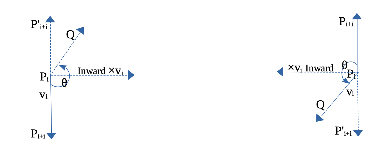
Fig. 79 Inward edge normals
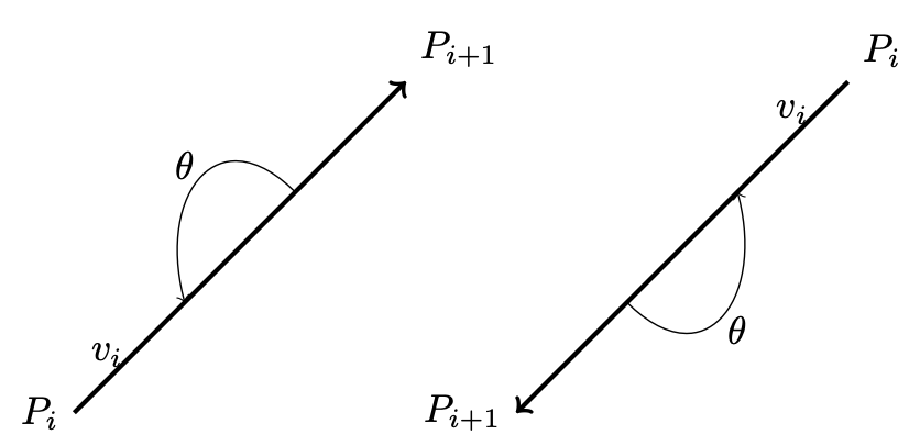
Fig. 80 Inward and outward in 2D for a vector.
Based on this observation, the rule for inward and outward vectors is shown in Fig. 79. Facing the same direction as a specific vector, the left side is inward and the right side is outward, as shown in Fig. 80.
For each edge \(P_i - P_{i+1}\), the inward edge normal is the vector \(\mathsf{x} \; v_i\); the outward edge normal is \(- \; \mathsf{x} \; v_i\), where \(\mathsf{x} \; v_i\) is the cross-product of \(v_i\), as shown in Fig. 79.
A polygon can be created from a set of vertices. Suppose \((P_0, P_1, ..., P_n)\) defines a polygon. The line segments \(P_0P_1, P_1P_2\), etc., are the polygon’s edges. The vectors \(v_0 = P_1 - P_0, v_1 = P_2 - P_1, ..., v_n = P_0 - P_n\) represent those edges.
Using counter-clockwise ordering, the left side is considered inward. Thus, the inward region of a polygon can be determined, as shown in Fig. 81 and Fig. 82.
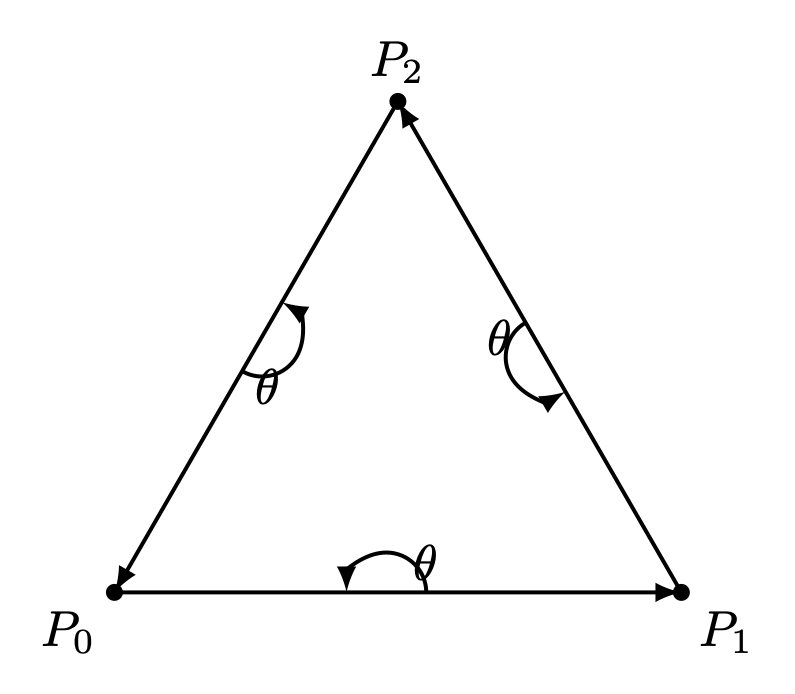
Fig. 81 Triangle with CCW¶ |
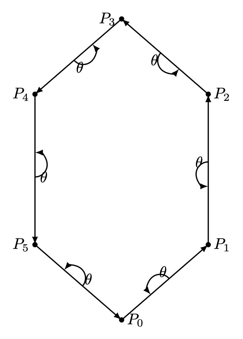
Fig. 82 Hexagon with CCW¶ |
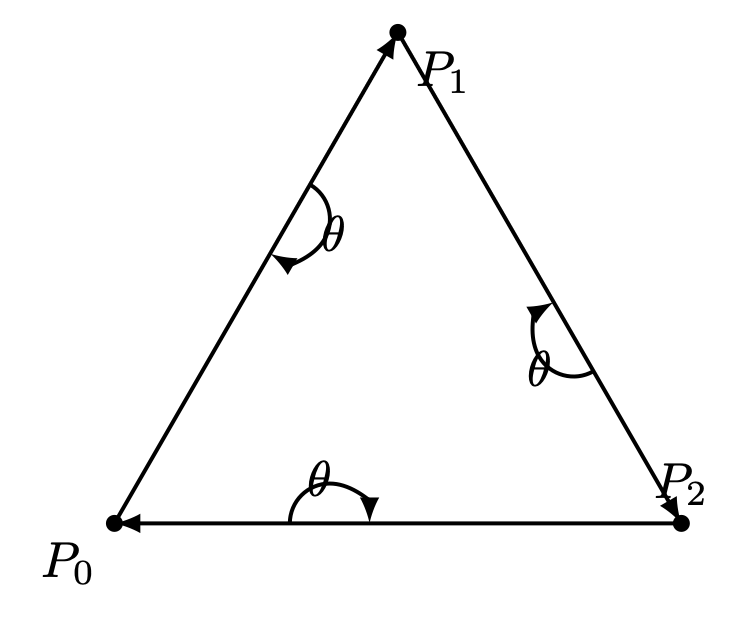
Fig. 83 Triangle with CW¶ |
For a convex polygon with vertices listed in counter-clockwise order, the inward edge normals point toward the interior of the polygon, and the outward edge normals point toward the unbounded exterior. This matches our usual intuition.
However, if the polygon vertices are listed in clockwise (CW) order, the interior and exterior definitions are reversed. Fig. 83 shows an example where \(P_0, P_1, P_2\) are arranged in CW order.
This cross product has an important property: going from \(v\) to \(\times v\) involves a 90° rotation in the same direction as the rotation from the positive x-axis to the positive y-axis.
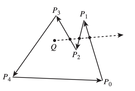
Fig. 84 Draw a polygon with vectices counter clockwise
As shown in Fig. 84, when drawing a polygon with vectors (lines) in counter-clockwise order, the polygon will be formed, and the two sides of each vector (line) can be identified [29].
Furthermore, whether a point is inside or outside the polygon can be determined.
One simple method to test whether a point lies inside or outside a simple polygon is to cast a ray from the point in any fixed direction and count how many times it intersects the edges of the polygon.
If the point is outside the polygon, the ray will intersect its edges an even number of times. If the point is inside the polygon, it will intersect the edges an odd number of times [30].
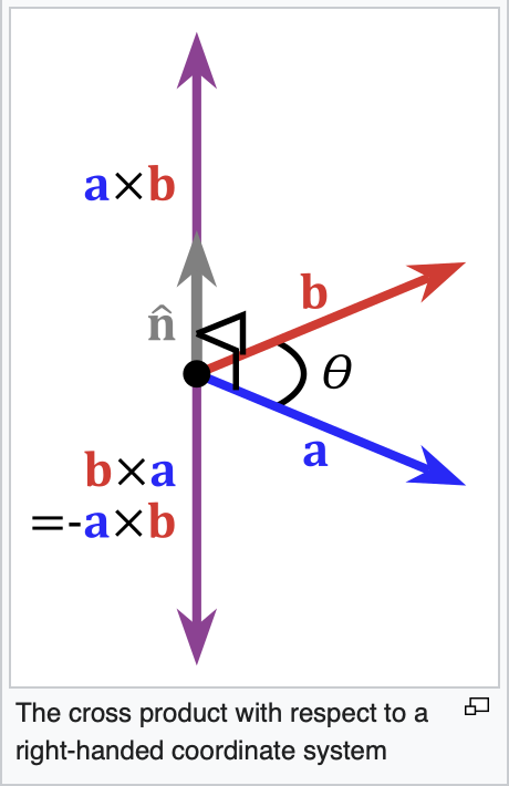
Fig. 85 Cross product definition in 3D
In the same way, by following the counter-clockwise direction to create a 2D polygon step by step, a 3D polygon can be constructed.
As shown in Fig. 85 from the wiki [26], the inward direction is determined by \(a \times b < 0\), and the outward direction is determined by \(a \times b > 0\) in OpenGL.
Replacing \(a\) and \(b\) with \(x\) and \(y\), as shown in Fig. 86, the positive Z-axis (\(z+\)) represents the outer surface, while the negative Z-axis (\(z-\)) represents the inner surface [31].
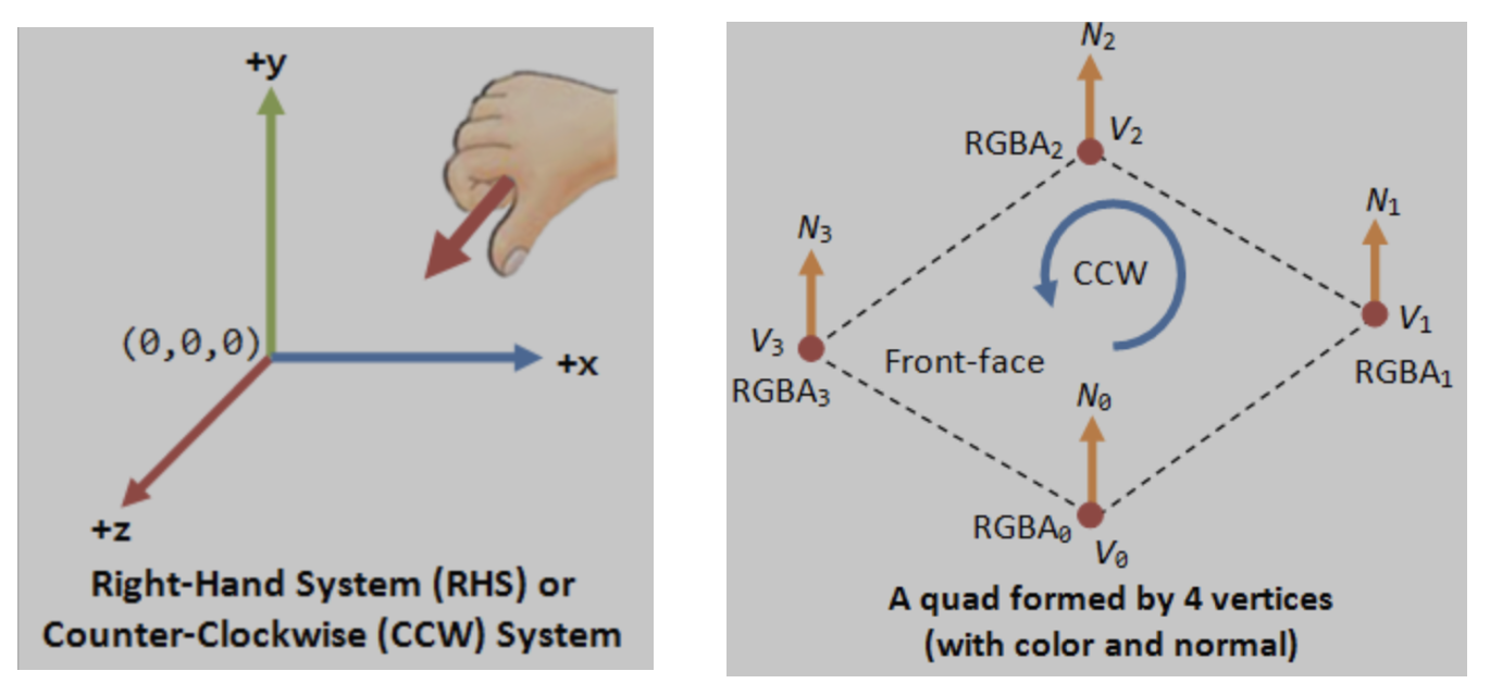
Fig. 86 OpenGL pointing outwards, indicating the outer surface (z axis is +)
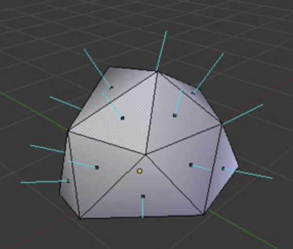
Fig. 87 3D polygon with directions on each plane
Reposition each triangle in front of camera and construct it using triangle with CCW ordering, as shown in Fig. 81. By building every triangle with CCW ordering, we can defined a consistent outer surface (front face). The Fig. 87 shows an example of a 3D polygon created from 2D triangles. The direction of the plane (triangle) is given by the line perpendicular to the plane.
Cast a ray from the 3D point along the X-axis and count how many intersections with the outer object occur. Depending on the number of intersections along each axis (even or odd), you can understan if the point (or the camara) is i nside or outside [32].
An odd number means inside, and an even number means outside. As shown in Fig. 88, points on the line passing through the object satisfy this rule.
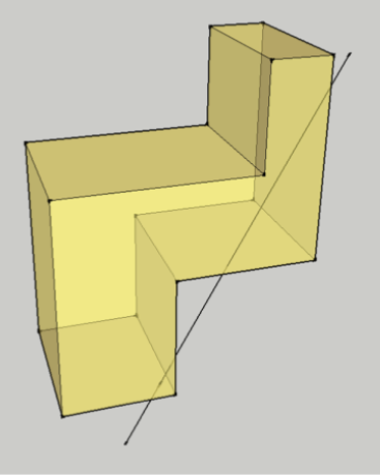
Fig. 88 Point is inside or outside of 3D object
✅ Summary:
Based on these description of this section, this means:
✔️ Each mesh (triangle or primitive) has a fixed “outer” and “inner” side, determined by CCW ordering in object space.
✔️ By reading these CCW-ordered vertices sequentially, the shape and surface orientation of the 3D model can be constructed.
✔️ There is no need to wait for the entire mesh to be received; once three CCW-ordered vertices are available, each triangle can be processed correctly as shown in Fig. 89 from the camera position \(p_0\).
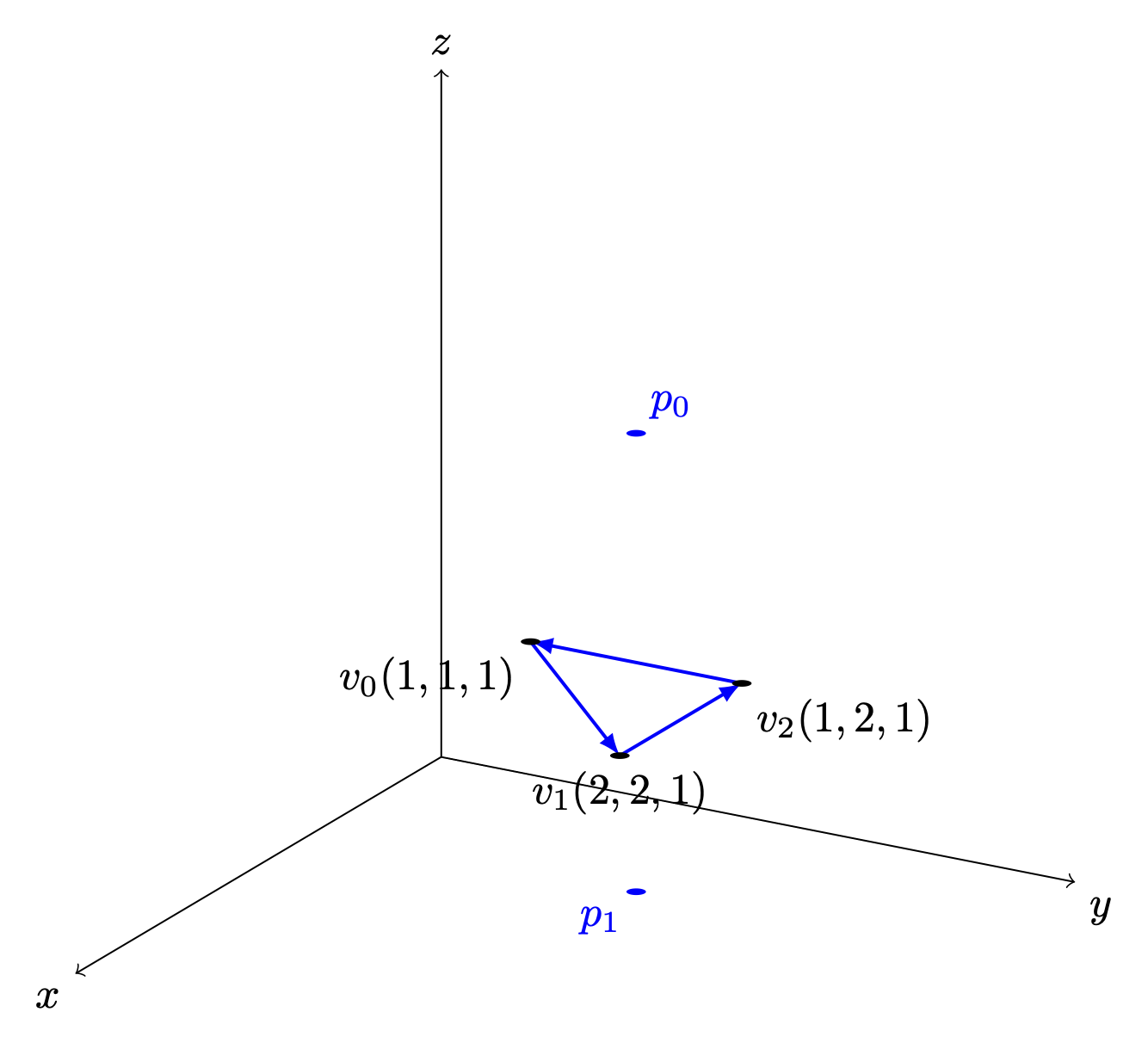
Fig. 89 A triangle can be constructed as soon as three vertices are received
✔️ When the camera moves to the \(p_1\) inside an object: CCW ↔ CW flips as shown in Fig. 89.
✔️ As shown in Trangle Area Calculation when \(0 < \Theta < 180^\circ\) under CCW orientation, the area of a triangle area is given by:
✔️ Though each triangle can be correctly identified and processed using its CCW ordering. As mentioned in Fig. 74 of section Transformation, the Cooridinates Transform Pipeline maps geometry from Camera Space to Clipping Space (Clipping Volume). This tranformation significantly simplifies the calculation required for discarding and clipping triangles, as will be desribed in the next section Projection.
How does OpenGL render (draw) the inner face of a triangle?
OpenGL does NOT determine front/back in world space.
When the camera moves to the inner space of a object:
The projection changes
The triangle’s screen‑space orientation changes
CCW ↔ CW flips
So the GPU flips front/back classification
OpenGL uses counter clockwise and pointing outwards as default [16].
// unit cube
// A cube has 6 sides and each side has 4 vertices, therefore, the total number
// of vertices is 24 (6 sides * 4 verts), and 72 floats in the vertex array
// since each vertex has 3 components (x,y,z) (= 24 * 3)
//    v6----- v5
//   /|      /|
//  v1------v0|
//  | |     | |
//  | v7----|-v4
//  |/      |/
//  v2------v3

// vertex position array
GLfloat vertices[]  = {
   .5f, .5f, .5f,  -.5f, .5f, .5f,  -.5f,-.5f, .5f,  .5f,-.5f, .5f, // v0,v1,v2,v3 (front)
   .5f, .5f, .5f,   .5f,-.5f, .5f,   .5f,-.5f,-.5f,  .5f, .5f,-.5f, // v0,v3,v4,v5 (right)
   .5f, .5f, .5f,   .5f, .5f,-.5f,  -.5f, .5f,-.5f, -.5f, .5f, .5f, // v0,v5,v6,v1 (top)
  -.5f, .5f, .5f,  -.5f, .5f,-.5f,  -.5f,-.5f,-.5f, -.5f,-.5f, .5f, // v1,v6,v7,v2 (left)
  -.5f,-.5f,-.5f,   .5f,-.5f,-.5f,   .5f,-.5f, .5f, -.5f,-.5f, .5f, // v7,v4,v3,v2 (bottom)
   .5f,-.5f,-.5f,  -.5f,-.5f,-.5f,  -.5f, .5f,-.5f,  .5f, .5f,-.5f  // v4,v7,v6,v5 (back)
};
From the code above, we can see that OpenGL uses counter-clockwise and
pointing outwards as the default. However, OpenGL provides
glFrontFace(GL_CW) for clockwise winding [33].
For a group of objects, a scene graph provides better animation support and saves memory [34].
Dot Product
Dot Product
Ray–plane (line–plane) intersection
Determining angles between vectors
Lighting (Lambertian shading)
Solving for a point on the intersection line of two planes (because plane equations use dot products)
Described in wiki here:
https://en.wikipedia.org/wiki/Dot_product
✅ As described in the previous section Cross Product, the cross-product is:
\(n\) is a unit vector perpendicular to the plane \(\Rightarrow\) direction.
The dot product definition is:
✅ Since \(n\) is the outward normal vector for a CCW-ordered triangle, we have:
\((\mathbf p - v_0) \mathsf \cdot \mathbf n > 0 \Rightarrow \mathbf p\) lies on the front (outer) side of the plane.
\((\mathbf p - v_0) \mathsf \cdot \mathbf n = 0 \Rightarrow \mathbf p\) lies on the plane.
\((\mathbf p - v_0) \mathsf \cdot \mathbf n < 0 \Rightarrow \mathbf p\) lies on the back (inner) side of the plane.
✅ A plane is represented by:
where:
\(n\) is the plane’s normal vector
\(x_0, x_1\) are any points on the plane
Let’s define the scalar constant \(d\) by:
Thus, the set of all points \(\mathbf{p}\) satisfying
✅ Ray–plane (line–plane) intersection
For an edge between vertices \(\mathbf{p}_0\) and \(\mathbf{p}_1\), parameterized as:
the intersection with a clipping plane is found by solving:
This yields:
Projection
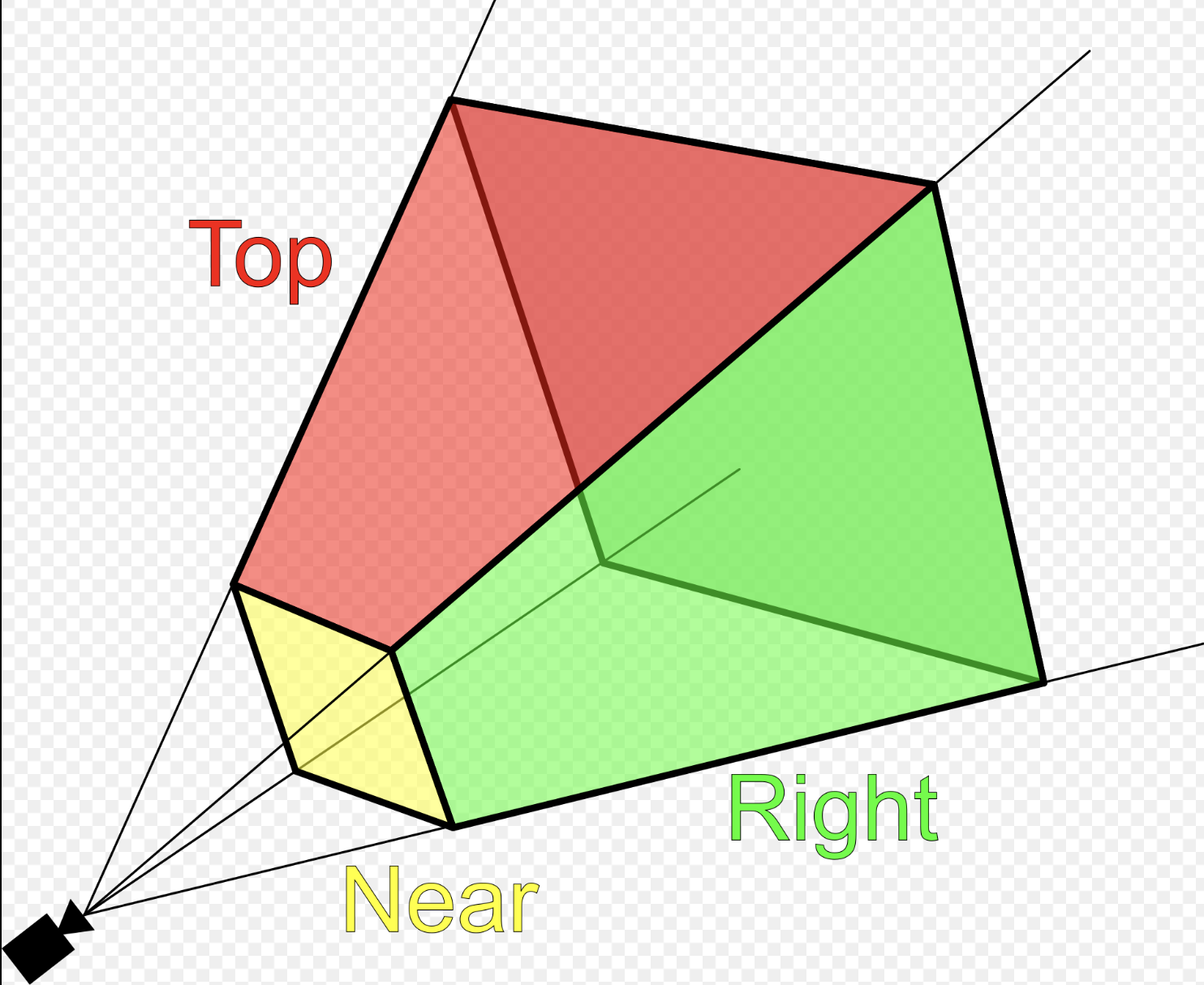
Fig. 90 Clipping-Volume Cuboid
Only objects within the cone between near and far planes are projected to 2D in perspective projection.
Perspective and orthographic projections (used in CAD tools) from 3D to 2D can be represented by transformation matrices as described in wiki here [25].
The “4.4 Projection Transform - Perspective Projection” of on the website [1] provides conceptual coverage of projections.
Camera Space Setup
Assume a right-handed camera coordinate system as shown in Fig. 90:
The camera is located at the origin.
The camera looks down the negative \(z\) axis.
The near plane is located at \(z = -n\).
The far plane is located at \(z = -f\).
The view frustum bounds on the near plane are:
left: \(l\)
right: \(r\)
bottom: \(b\)
top: \(t\)
A point in camera space is represented as:
The position on the near plane is:
✅ Reason:
As described in the previous section Cross Product, each mesh (triangle or primitive) has a fixed “outer” and “inner” side, determined by CCW ordering in object space. By reading these CCW-ordered vertices sequentially, the shape and surface orientation of the 3D model can be constructed, and hidden primitives can be clipped or discarded.
However primitive clipping and discarding can be performed much more efficiently by mapping the view frustum to clip space, where the GPU can easily clip or discard primitives, as shown Fig. 91 from the earlier section Transformation again for clarity. Performing clipping and discarding in world space would be significantly more difficult.
Perspective projection \(P_{\text{persp}}\) (general form): Converts 3D → clip space with depth
by a homogeneous point
Converting from camera space to cliping space produces a homogeneous coordinate of the form \([x, y, z, w_c]\):
After transforming to ciip space, each vertex corrodinate is expressed in homogeneous form, and the view frustum boundaries are encoded in the coordinate values. A vertex lies inside the view frustum if the following conditions are satisfied:
The near plane is located at \(z = -n\). When \(w_c = -n\), the geometry is mapped to the normalized device coordinates (NDC) on the screen.
After perspective division —- that is, dividing clip-space coordinates by \(w_c = -n\) —- the resulting NDC are:
This matrix maps the view frustum in camera space to the normalized cube in NDC after homogeneous division.
✅ Comparsion for clipping and discarding in World Space and Clipping Space
When a triangle intersects the view frustum, it must be clipped so that only the portion inside the frustum is rasterized. Although the clipping procedure is conceptually similar in world space and clip space, the mathematical complexity differs significantly. Clipping and discarding in clip space will saves 85% in instructions.
1A. Discarding in world space:
As described in the section Dot Product:
The definition of Dot Product is:
When \((\mathbf p - v_0) \mathsf \cdot \mathbf n < 0 \Rightarrow \mathbf p\) lies on the back (inner) side of the plane.
For the ray–plane (line–plane) intersection, the \(d_i\) can be obtained by choosing any point \(\mathbf{p}_0\) on the plane with normal vector \(\mathbf{n}_i\).
In world (or view) space, the view frustum is bounded by six arbitrary planes, each defined by a normal vector \(\mathbf{n}\) and distance \(d\).
For each vertex \(\mathbf{p}\), discarding requires testing against all planes:
Cost per vertex
6 dot products (each ≈ 3 multiplications + 2 additions)
6 additions with plane constants
6 comparisons
Approximate arithmetic cost:
18 multiplications
18 additions
6 comparisons
1B. Discarding in clip space:
In clip space, vertices are represented in homogeneous coordinates \((x_c, y_c, z_c, w_c)\). The view frustum becomes an axis-aligned volume defined by:
Approximate arithmetic cost:
6 comparisons
Overall arithmetic instruction reduction 85% ~ 95%.
2A. Clipping in World Space:
Edge–plane intersection
As described in the section Dot Product, the ray–plane (line–plane) intersection can be derived as follows:
Each frustum plane requires a separate equation and dot-product evaluation.
Triangle reconstruction
After computing all intersection points:
New vertices are inserted along intersecting edges
The original triangle is split into one or more triangles
Perspective projection is applied afterward
Care must be taken to preserve perspective correctness during interpolation.
2B. Clipping in Clip Space:
Edge–plane intersection
Edges are interpolated linearly in homogeneous space:
Intersection with a clipping boundary is found by solving equations such as:
Each case reduces to a single scalar equation for \(t\).
Compare \(t = \frac{x_0 - w_0}{(x_0 - w_0) - (x_1 - w_1)}\) and the equation from world space \(t = \frac{- (\mathbf{n} \cdot \mathbf{p}_0 + d)}{\mathbf{n} \cdot (\mathbf{p}_1 - \mathbf{p}_0)}\), it saves 85% for reducing two dot operations and more opertions.
Triangle reconstruction
After clipping:
New vertices remain in homogeneous coordinates
Perspective division is deferred
Linear interpolation remains perspective-correct
The final step applies the perspective divide:
4.3 Comparison and Practical Implications
World-space clipping and discarding uses general plane equations and complex geometry.
Clip-space clipping and discarding uses axis-aligned bounds and simple interpolation.
Perspective correctness is naturally preserved in clip space.
GPU hardware can implement clip-space clipping and discarding efficiently.
For these reasons, modern graphics pipelines perform triangle clipping and discarding in clip space, not in world space.
✅ Perspective Projection Matrix Derivation
This section derives the perspective projection matrix by mapping a view frustum in camera space to Normalized Device Coordinates (NDC).
A vertex is kept only if it satisfies the following inequalities:
These inequalities define the view frustum in homogeneous coordinates.
If a vertex violates any of these conditions, it lies outside the view frustum (left, right, top, bottom, near, or far plane) and is clipped or discarded.
The goal is to map this frustum to Normalized Device Coordinates (NDC):
Homogeneous Perspective Divide
After projection, homogeneous division is applied:
To achieve perspective foreshortening, the homogeneous coordinate must satisfy:
This requirement determines the last row of the projection matrix.
X Coordinate Mapping
By similar triangles, the projected x-coordinate on the near plane is:
The near-plane bounds map to NDC as follows:
Assume a linear mapping:
Applying the near constraints: substituting \(x_n = l\ and\ x_{ndc} = -1\):
Applying the far constraints: substituting \(x_n = r\ and\ x_{ndc} = 1\):
Solving equations (1) and (2) to get \(A_x\):
Substituting equation (3) to (2):
From (3) and (4): Solving for \(A_x\) and \(B_x\) yields:
Substituting \(x_n\) gives the resulting mapping is:
Y Coordinate Mapping:
Using the same derivation for the y-axis:
The resulting mapping is:
Z Coordinate Mapping
Depth is mapped linearly such that:
Assume:
Then:
Applying the near constraints: substituting \(z = -n\ and\ z_{ndc} = -1\):
Applying the far constraints: substituting \(z = -f\ and\ z_{ndc} = 1\):
Solving equations (1) and (2) to get \(A_z\):
Substituting equation (3) to (2):
From (3) and (4):
Perspective Projection Matrix
Combining all components, the perspective projection matrix is:
Projection: The explanation and mathematical proof is given below also.
Reference:
1. Every computer graphics book covers the topic of transformation of objects and their positions in space. Chapter 4 of the Blue Book: OpenGL SuperBible, 7th Edition provides a concise yet useful 40-page overview of transformation concepts and is good material for gaining a deeper understanding of transformations. description of transformation.
Chapter 7 of Red book covers the tranformations and projections.
OpenGL
Example of OpenGL program
The following example is from the OpenGL Red Book and its example code [37] [43].
References/triangles.vert
#version 400 core

layout( location = 0 ) in vec4 vPosition;

void
main()
{
    gl_Position = vPosition;
}
References/triangles.frag
#version 450 core

out vec4 fColor;

void main()
{
    fColor = vec4(0.5, 0.4, 0.8, 1.0);
}
References/01-triangles.cpp
  1//////////////////////////////////////////////////////////////////////////////
  2//
  3//  Triangles.cpp
  4//
  5//////////////////////////////////////////////////////////////////////////////
  6
  7#include "vgl.h"
  8#include "LoadShaders.h"
  9
 10enum VAO_IDs { Triangles, NumVAOs };
 11enum Buffer_IDs { ArrayBuffer, NumBuffers };
 12enum Attrib_IDs { vPosition = 0 };
 13
 14GLuint  VAOs[NumVAOs];
 15GLuint  Buffers[NumBuffers];
 16
 17const GLuint  NumVertices = 6;
 18
 19//----------------------------------------------------------------------------
 20//
 21// init
 22//
 23
 24void
 25init( void )
 26{
 27    glGenVertexArrays( NumVAOs, VAOs ); // Same with glCreateVertexArray( NumVAOs, VAOs );
 28      // https://stackoverflow.com/questions/24441430/glgen-vs-glcreate-naming-convention
 29    // Make the new VAO:VAOs[Triangles] active, creating it if necessary.
 30    glBindVertexArray( VAOs[Triangles] );
 31    // opengl->current_array_buffer = VAOs[Triangles]
 32
 33    GLfloat  vertices[NumVertices][2] = {
 34        { -0.90f, -0.90f }, {  0.85f, -0.90f }, { -0.90f,  0.85f },  // Triangle 1
 35        {  0.90f, -0.85f }, {  0.90f,  0.90f }, { -0.85f,  0.90f }   // Triangle 2
 36    };
 37
 38    glCreateBuffers( NumBuffers, Buffers );
 39
 40    // Make the buffer the active array buffer.
 41    glBindBuffer( GL_ARRAY_BUFFER, Buffers[ArrayBuffer] );
 42    // Attach the active VBO:Buffers[ArrayBuffer] to VAOs[Triangles]
 43    // as an array of vectors with 4 floats each.
 44    // Kind of like:
 45    // opengl->current_vertex_array->attributes[attr] = {
 46    //     type = GL_FLOAT,
 47    //     size = 4,
 48    //     data = opengl->current_array_buffer
 49    // }
 50    // Can be replaced with glVertexArrayVertexBuffer(VAOs[Triangles], Triangles,
 51    // buffer[ArrayBuffer], ArrayBuffer, sizeof(vmath::vec2));, glVertexArrayAttribFormat(), ...
 52    // in OpenGL 4.5.
 53
 54    glBufferStorage( GL_ARRAY_BUFFER, sizeof(vertices), vertices, 0);
 55
 56    ShaderInfo  shaders[] =
 57    {
 58        { GL_VERTEX_SHADER, "media/shaders/triangles/triangles.vert" },
 59        { GL_FRAGMENT_SHADER, "media/shaders/triangles/triangles.frag" },
 60        { GL_NONE, NULL }
 61    };
 62
 63    GLuint program = LoadShaders( shaders );
 64    glUseProgram( program );
 65
 66    glVertexAttribPointer( vPosition, 2, GL_FLOAT,
 67                           GL_FALSE, 0, BUFFER_OFFSET(0) );
 68    glEnableVertexAttribArray( vPosition );
 69    // Above two functions specify vPosition to vertex shader at layout (location = 0)
 70}
 71
 72//----------------------------------------------------------------------------
 73//
 74// display
 75//
 76
 77void
 78display( void )
 79{
 80    static const float black[] = { 0.0f, 0.0f, 0.0f, 0.0f };
 81
 82    glClearBufferfv(GL_COLOR, 0, black);
 83
 84    glBindVertexArray( VAOs[Triangles] );
 85    glDrawArrays( GL_TRIANGLES, 0, NumVertices );
 86}
 87
 88//----------------------------------------------------------------------------
 89//
 90// main
 91//
 92
 93#ifdef _WIN32
 94int CALLBACK WinMain(
 95  _In_ HINSTANCE hInstance,
 96  _In_ HINSTANCE hPrevInstance,
 97  _In_ LPSTR     lpCmdLine,
 98  _In_ int       nCmdShow
 99)
100#else
101int
102main( int argc, char** argv )
103#endif
104{
105    glfwInit();
106
107    GLFWwindow* window = glfwCreateWindow(800, 600, "Triangles", NULL, NULL);
108
109    glfwMakeContextCurrent(window);
110    gl3wInit();
111
112    init();
113
114    while (!glfwWindowShouldClose(window))
115    {
116        display();
117        glfwSwapBuffers(window);
118        glfwPollEvents();
119    }
120
121    glfwDestroyWindow(window);
122
123    glfwTerminate();
124}
Init():
Generate Vertex Array VAOs and bind VAOs[0].
(glGenVertexArrays(NumVAOs, VAOs); glBindVertexArray(VAOs[Triangles]); glCreateBuffers(NumBuffers, Buffers);)
A vertex-array object holds various data related to a collection of vertices. Those data are stored in buffer objects and managed by the currently bound vertex-array object.
glBindBuffer(GL_ARRAY_BUFFER, Buffers[ArrayBuffer]);
Because there are many different places where buffer objects can be in OpenGL, when we bind a buffer, we need to specify what we’d like to use it for. In our example, because we’re storing vertex data into the buffer, we use GL_ARRAY_BUFFER. The place where the buffer is bound is known as the binding target.
According to the counter-clockwise rule in the previous section, triangle primitives are defined in variable vertices. After binding OpenGL VBO Buffers[0] to vertices, vertex data will be sent to the memory of the server (GPU).
Think of the “active” buffer as just a global variable, and there are a bunch of functions that use the active buffer instead of taking using a parameter. These global state variables are the ugly side of OpenGL [44] and can be replaced with glVertexArrayVertexBuffer(), glVertexArrayAttribFormat(), etc. Then call glBindVertexArray(vao) before drawing in OpenGL 4.5 [45] [46].
glVertexAttribPointer(vPosition, 2, GL_FLOAT, GL_FALSE, 0, BUFFER_OFFSET(0)):
During GPU rendering, each vertex position will be held in vPosition and passed to the “triangles.vert” shader through the LoadShaders(shaders) function.
glfwSwapBuffers(window):
You’ve already used double buffering for animation. Double buffering is done by making the main color buffer have two parts: a front buffer that’s displayed in your window; and a back buffer, which is where you render the new image. When you swap the buffers (by calling glfwSwapBuffers(), for example), the front and back buffers are exchanged [86].
display():
Bind VAOs[0], set render mode to GL_TRIANGLES and send vertex data to Buffer (gpu memory, OpenGL pipeline). Next, GPU will do rendering pipeline descibed in next section.
The triangles.vert has input vPosition and no output variable, so using gl_Position default varaible without declaration. The triangles.frag has not defined input variable and has defined output variable fColor instead of using gl_FragColor.
The “in” and “out” in shaders above are “type qualifier”. A type qualifier is used in the OpenGL Shading Language (GLSL) to modify the storage or behavior of global and locally defined variables. These qualifiers change particular aspects of the variable, such as where they get their data from and so forth [51].
Though attribute and varying are removed from later version 1.4 of OpenGL, many materials in website using them [52] [53]. It’s better to use “in” and “out” to replace them as the following code. OpenGL has a few ways to binding API’s variable with shader’s variable. glVertexAttrib* as the following code and glBindAttribLocation() [54], …
replace attribute and varying with in and out
uniform float scale;
layout (location = 0) attribute vec2 position;
// layout (location = 0) in vec2 position;
layout (location = 1) attribute vec4 color;
// layout (location = 1) in vec4 color;
varying vec4 v_color;
// out v_color

void main()
{
  gl_Position = vec4(position*scale, 0.0, 1.0);
  v_color = color;
}
// OpenGL API
GLfloat attrib[] = { x * 0.5f, x * 0.6f, x* 0.4f, 0.0f };
// Update the value of input attribute 1 : layout (location = 1) in vec4 color
glVertexAttrib4fv(1, attrib);
varying vec4 v_color;
// in vec4 v_color;

void main()
{
  gl_FragColor = v_color;
}
An OpenGL program is made of two shaders [49] [50]:
The vertex shader is (commonly) executed once for every vertex we want to draw. It receives some attributes as input, computes the position of this vertex in space and returns it in a variable called gl_Position. It also defines some varyings.
The fragment shader is executed once for each pixel to be rendered. It receives some varyings as input, computes the color of this pixel and returns it in a variable called fColor.
Since we have 6 vertices in our buffer, this shader will be executed 6 times by the GPU (once per vertex)! We can also expect all 6 instances of the shader to be executed in parallel, since a GPU have so many cores.
3D Rendering
3D animation is the process of creating moving images by manipulating digital objects within a three‑dimensional space. 3D rendering is the process of converting 3D models into 2D images on a computer [35].
Based on the previous section of 3D modeling, the 3D modeling tool will generate a 3D vertex model and OpenGL code. Then, programmers may manually modify the OpenGL code and add or update shaders.
In section SW Stack and Data Flow, we mentioned the GPU will generate the rendering image for each frame according the 3D Inforamtion and Uniform Updates sent from CPU, and write each of the final frame of data in the form of color pixels to framebuffer (video memory) as Fig. 69.
Animation Parameters
✅ CPU only updates small animation parameters named Uniform Updates as appeared in Fig. 68; GPU computes the heavy per‑vertex work.
The 3D animation will trigger the 3D rendering process for each 2D image drawing accoriding the Uniform Updates.
The “small animation parameters” updated by the CPU are formally called:
✔ Uniform updates
✔ Constant buffer updates
✔ Per‑frame / per‑draw constants
✔ Bone matrix palette updates (for skinning)
✔ Morph weight updates (for morphing)
These are the correct technical terms used in modern graphics pipelines.
⚓ The Proper Term: “Uniform Updates”
The most accurate and universal name is:
✅ Uniform updates
or
✅ Updating uniform buffers
Because the CPU is updating uniform data that the GPU reads during shading.
Examples of uniform data:
bone matrices
morph weights
animation time
material parameters
camera matrices
light parameters
These are small, constant‑for‑the‑draw values.
⚓ More Specific Terms Used in Game Engines
Animation Parameters
Used in animation systems:
“animation parameters”
“skinning parameters”
“bone palette”
“morph weights”
Per‑Frame Constants
Used in engine architecture:
“frame constants”
“per‑frame constant buffer”
“global shader constants”
Per‑Draw Constants
Used in render pipelines:
“per‑draw uniform block”
“per‑object constant buffer”
“material constant buffer”
⚓ In Modern APIs (GL, Vulkan, DirectX)
OpenGL
Uniforms
Uniform Buffer Objects (UBOs)
Shader Storage Buffer Objects (SSBOs)
DirectX
Constant Buffers (CBuffers)
Vulkan
Descriptor sets
Uniform buffers
All refer to the same concept: small CPU‑updated data that the GPU reads during shading.
3D Rendering Pipeline
The steps are shown in Fig. 92.
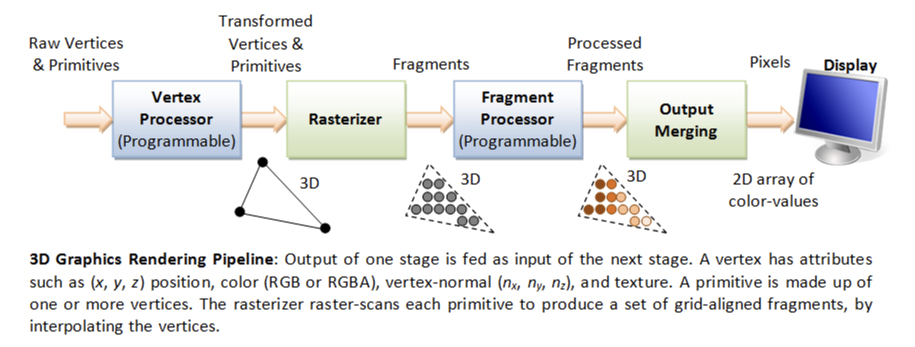
A fragment can be treated as a pixel in 3D spaces, which is aligned with the pixel grid, with attributes such as position, color, normal and texture.
From the previous Fig. 68 and Fig. 69 in section SW Stack and Data Flow, we introduce the 3D anmiation data are classified as follows:
Vertex Data = 3D model information (the mesh (geometry), such as VBO/VAO)
Animation Parameters = per‑frame uniform updates (transforms, bone matrices, camera, materials, …)
The complete steps of 3D Rendering pipeline, excluding animation are shown in the Fig. 93 from the OpenGL website [36] and in the Fig. 94. The website also provides a description for each stage. To clarify the modern GPU pipeline, Fig. 95 shows the use of Primitive Assembly (fixed-function) and Primitive Setup (fixed-function).
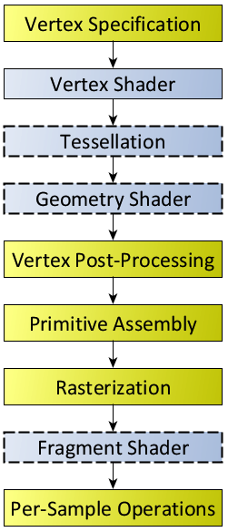
Fig. 93 Diagram of the Rendering Pipeline. The blue boxes are programmable shader stages. Shaders with dashed outlines indicate optional shader stages.¶ |
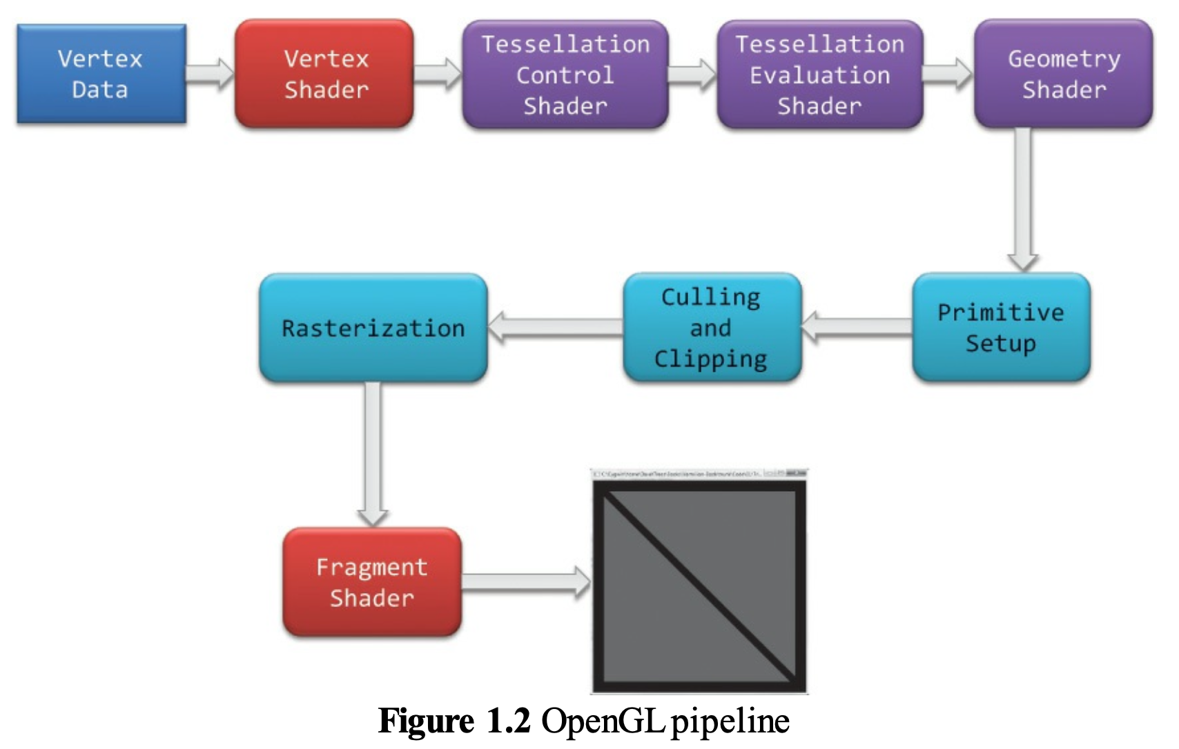
Fig. 94 OpenGL pipeline in blue book¶ |
![digraph GPU_Pipeline {
rankdir=LR;
node [shape=box, style=rounded, fontsize=12];
VB [label="Vertex Buffer"];
VS [label="Vertex Shader", style=filled, fillcolor=orange];
subgraph cluster_ts {
label="Tessellation";
style=rounded;
TCS [label="Tessellation\nControl Shader\n(optional)", style=filled, fillcolor=orange];
TS [label="Tessellator\n(fixed-function)"];
TES [label="Tessellation\nEvaluation Shader\n(optional)", style=filled, fillcolor=orange];
{ rank = same; TCS; TS; TES }
}
subgraph cluster_pp {
label="Primitive Processing";
style=rounded;
PA [label="Primitive Assembly\n(topology formation)"];
GS [label="Geometry Shader\n(optional)", style=filled, fillcolor=orange];
Cull [label="Culling"];
Clip [label="Clipping"];
PS [label="Primitive Setup\n(rasterization\n prep)"];
{ rank = same; PA; GS; Cull; Clip; PS }
}
RAST [label="Rasterizer"];
FS [label="Fragment Shader", style=filled, fillcolor=orange];
FB [label="Framebuffer"];
VB -> VS;
VS -> TCS;
TCS -> TS;
TS -> TES;
// Bypass tessellation path
VS -> PA [label="(no tessellation)", style=dashed];
TES -> PA;
PA -> GS [label = "Primitives\n(triangles/lines)"];
GS -> Cull;
Cull -> Clip;
Clip -> PS;
PS -> RAST;
RAST -> FS;
FS -> FB;
{ rank = same; FS; FB }
}](_images/graphviz-b2f5f932bdb3689e8c7f4cdd4f7b1a113dfa63a4.png)
Fig. 95 Modern GPU Pipeline
As shown in Fig. 95:
Vertex Shader and Tessellation: processing and transform for vertices data.
Primitive Processing: processing and transform for primitives data.
Rasterizer: Primitives → Fragment.
Fragment Shader: Fragment → Colored Fragment.
As illustred in Cross Product section,
✔️ Each mesh (triangle or primitive) has a fixed “outer” and “inner” side, determined by CCW ordering in object space.
✔️ By reading these CCW-ordered vertices sequentially, the shape and surface orientation of the 3D model can be constructed.
✔️ There is no need to wait for the entire mesh to be received; once three CCW-ordered vertices are available, each triangle can be processed correctly.
✔️ When the camera moves to the inside an object: CCW ↔ CW flips.
This means:
✔️ Vertex Shader and Tessellation: may processing each vertex independently as long as the vertex order is preserved.
✔️ Once three CCW-ordered vertices are available, Primitive Assembly can convert them into a triangle and pass it to the next pipeline stage.
For example: once v0,v1,v2,v3 are available, Primitive Assembly outputs:
Triangle A (v0,v1,v2)
Triangle B (v2,v3,v0)
After vertices are assembled into primitives (such as triangles), the front-facing and back-facing surfaces can be determined, and the hidden primitives can be removed.
The Red Book and Blue Book show only Vertex Specification and Vertex Data in the rendering flow because they never show Animation Parameters as part of the rendering flow. The animation flow from CPU to GPU is shown in Fig. 96, based on Fig. 92.
![digraph CPU_GPU_Pipeline {
rankdir=LR;
node [shape=box, style=rounded, fontsize=12];
subgraph cluster_cpu {
label="CPU";
style=rounded;
CPU_Vertex [label="Load 3D Model\n(Vertex Data)\nVBOs, VAOs, Indices"];
CPU_Anim [label="Update Animation Parameters\n(Bone Matrices, Morph Weights,\nTime, Material Params)"];
}
subgraph cluster_gpu {
label="GPU";
style=rounded;
VS [label="Vertex Shader\n(Skinning, Morphing,\nModel/View/Proj Transform)"];
Raster [label="Rasterizer\n(Primitive Assembly,\nClipping, Interpolation)"];
FS [label="Fragment Shader\n(Lighting, Texturing,\nShading, Materials)"];
FB [label="Final Rendered Image\n(Framebuffer Output)"];
}
CPU_Vertex -> VS;
CPU_Anim -> VS;
VS -> Raster;
Raster -> FS;
FS -> FB;
}](_images/graphviz-bb6f73a70da9de0610bb1f0a2887d215e8cf21b1.png)
Fig. 96 CPU and GPU Pipeline For Shaders
Each draw call may correspond to:
one mesh
one submesh
one meshlet (in mesh‑shader pipelines)
or many meshes batched together
Although the Rendering Pipeline shown in Fig. 93 and Fig. 94 do not explicitly include per-frame animation flow— because the inputs are labeled Vertex Specification and Vertex Data and they do not show Animation Parameters as part of the rendering process—the pipeline is still applicable.
However the following table from OpenGL rendering pipeline Figure 1.2 and its stages from the book OpenGL Programming Guide, 9th Edition [37] is broad enough to cover animation.
Stage. |
Description |
|---|---|
Vertex Shading |
Vertex → Vertex and other data such as color for later passes. For each vertex issued by a drawing command, a vertex shader processes the data associated with that vertex. Vertex Shader: provides the Vertex → Vertex transformation effects controlled by the users. |
Tessellation Shading |
Create more detail on demand when zoomed in. After the vertex shader processes each vertex, the tessellation shader stage (if active) continues processing. The tessellation stage is actually divided into two shaders known as the tessellation control shader and the tessellation evaluation shader. A single patch from Tesslation Control Shader (TCS) and Tesslation Evaluation Shader (TVS) can generate millions of micro‑triangles. See reference below. |
Primitive Assembly |
This is a fixed‑function hardware stage: forms triangles/lines/points. |
Geometry Shader |
Primitive Transformation: output zero primitives (cull), output one primitive (pass‑through), output many primitives (amplify) and output different topology (e.g., point → quad) Allows additional processing of geometric primitives. This stage may create new primitives before rasterization. The Geometry shading stage is another optional stage that can modify entire geometric primitives within the OpenGL pipeline. This stage operates on individual geometric primitives allowing each to be modified. In this stage, you might generate more geometry from the input primitive, change the type of geometric primitive (e.g., converting triangles to lines), or discard the geometry altogether. |
Culling |
Remove entire primitives that are hidden or outside the viewport. |
Clipping |
Clip the hidden portions of the primitive, separating it into visible and hidden parts and discarding the hidden portions. |
Primitive Setup (rasterization preparation) |
This stage: takes the final primitive (after GS), computes edge equations, computes barycentric interpolation coefficients, determine rasterization rules and prepare for triangle traversal. |
Rasterization |
Geometric Primitives → Fragment. The job of the rasterizer is to determine which screen locations are covered by a particular piece of geometry (point, line, or triangle). Knowing those locations, along with the input vertex data, the rasterizer linearly interpolates the data values for each varying variable in the fragment shader and sends those values as inputs into your fragment shader. A fragment can be treated as a pixel in 3D spaces, which is aligned with the pixel grid, with attributes such as position, color, normal and texture. Early Depth and Stencil Tests (Early‑Z): reject hidden fragments before shading. |
Fragment Shading |
Fragment → Colored Fragment. Determine color for each pixel. In this stage, a fragment’s color and depth values are computed and then sent for further processing in the fragment-testing and blending parts of the pipeline. The final stage where you have programmable control over the color of a screen location is fragment shading. In this shader stage, you use a shader to determine the fragment’s final color (although the next stage, per-fragment operations, can modify the color one last time) and potentially its depth value. Fragment shaders are very powerful, as they often employ texture mapping to augment the colors provided by the vertex processing stages. A fragment shader may also terminate processing a fragment if it determines the fragment shouldn’t be drawn; this process is called fragment discard. A helpful way of thinking about the difference between shaders that deal with vertices and fragment shaders is this: vertex shading (including tessellation and geometry shading) determines where on the screen a primitive is, while fragment shading uses that information to determine what color that fragment will be. |
Stage. |
Description |
|---|---|
Per-Fragment Operations |
During this stage, a fragment’s visibility is determined using depth testing (also commonly known as z-buffering) and stencil testing. If a fragment successfully makes it through all of the enabled tests, it may be written directly to the framebuffer, updating the color (and possibly depth value) of its pixel, or if blending is enabled, the fragment’s color will be combined with the pixel’s current color to generate a new color that is written into the framebuffer. |
Compute shading stage |
Compute shader: may be applied in any stage. This is not part of the graphical pipeline like the stages above, but stands on its own as the only stage in a program. A compute shader processes generic work items, driven by an application-chosen range, rather than by graphical inputs like vertices and fragments. Compute shaders can process buffers created and consumed by other shader programs in your application. This includes framebuffer post-processing effects or really anything you want. Compute shaders are described in Chapter 12 of Red Book, “Compute Shaders” [40]. |
Tessllation
Tessellation Shading: The core problem that Tessellation deals with is the static nature of 3D models in terms of their detail and polygon count. The thing is that when we look at a complex model such as a human face up close we prefer to use a highly detailed model that will bring out the tiny details (e.g. skin bumps, etc). A highly detailed model automatically translates to more triangles and more compute power required for processing. … One possible way to solve this problem using the existing features of OpenGL is to generate the same model at multiple levels of detail (LOD). For example, highly detailed, average and low. We can then select the version to use based on the distance from the camera. This, however, will require more artist resources and often will not be flexible enough. … Let’s take a look at how Tessellation has been implemented in the graphics pipeline. The core components that are responsible for Tessellation are two new shader stages and in between them a fixed function stage that can be configured to some degree but does not run a shader. The first shader stage is called Tessellation Control Shader (TCS), the fixed function stage is called the Primitive Generator (PG), and the second shader stage is called Tessellation Evaluation Shader (TES). Some GPU havn’t this fixed function stage implemented in HW and even havn’t provide these TCS, TES and Gemoetry Shader. User can write Compute Shaders instead for this on-fly detail display. This surface is usually defined by some polynomial formula and the idea is that moving a CP has an effect on the entire surface. … The group of CPs is usually called a Patch [38]. The data flow in Tessllation Stage between TCS, Fixed-Function Tessellator and TES is illustrated in Fig. 97. Chapter 9 of Red Book [37] has details. The next section Tessellation Example describes the details for the Tessallation with an example.
Tessellation cannot decrease the resolution of vertices from the VS. The Geometry Shader can reduce geometry (by discarding primitives), but it cannot reduce the number of input vertices coming from VS/TES. The rasterizer can reduce fragments, but it cannot reduce vertices.
Data Flow
Sumarize the OpenGL Rendering Pipeline as shown in the Fig. 97 and Fig. 98.
![digraph OpenGL_Pipeline_Part1 {
rankdir=LR;
node [shape=box, style=rounded, fontsize=12];
App [label="Application"];
VS [label="Vertex Shader"];
subgraph cluster_optional {
label="Optional Stages";
style="rounded,dashed";
color="gray";
subgraph cluster_ts {
label="Tessellation";
style=rounded;
TCS [label="Tessellation Control Shader\n(TCS)"];
TS [label="Fixed-Function Tessellator"];
TES [label="Tessellation Evaluation Shader\n(TES)"];
TCS -> TS [label="CP + Tessellation level"];
TS -> TES [label="Tessellated domain\ncoordinates"];
{ rank = same; TCS; TS; TES }
}
GS [label="Geometry Shader"];
}
PA [label="Primitive Assembly"];
PS [label="Primitive Setup"];
App -> VS [label="Vertex Arrays"];
VS -> TCS [label="Transformed Vertices +\nControl Points(CP)"];
TES -> PA [label="Tessellated Vertices\n(more vertices)"];
PA -> GS;
GS -> PS [label="Modified Primitives"];
//{ rank = same; TCS; TES }
}](_images/graphviz-4d3a954b93b61e73796fc6f5a43463b86c857fc8.png)
Fig. 97 The part 1 of GPU Rendering Pipeline Stages
![digraph OpenGL_Pipeline_Part2 {
rankdir=LR;
node [shape=box, style=rounded, fontsize=12];
PS [label="Primitive Setup"];
Raster [label="Rasterization"];
FS [label="Fragment Shader"];
PF [label="Per-Fragment Ops"];
FB [label="Framebuffer"];
PS -> Raster [label="Assembled Primitives"];
Raster -> FS [label="Fragments"];
FS -> PF [label="Colored Fragments"];
PF -> FB [label="Final Fragments"];
}](_images/graphviz-14c4dabc0c0ae177af778c933c3bf996965eca2d.png)
Fig. 98 The part 2 of GPU Rendering Pipeline Stages
The data flow through the OpenGL Shader and the details flow in TCS, Fixed-Function Tessellator and TES are described in below.
Shader Stage |
Input Data (from CPU or previous stage) |
Output Data (to next stage) |
How GPU Hardware Uses These Data (with Stage Name) |
|---|---|---|---|
Vertex Shader |
|
|
|
Tessellation Control Shader (TCS) |
|
|
|
Fixed‑Function Tessellator (TS) |
|
|
|
Tessellation Evaluation Shader (TES) |
|
|
|
Geometry Shader |
|
|
|
Shader Stage |
Input Data (from CPU or previous stage) |
Output Data (to next stage) |
How GPU Hardware Uses These Data (with Stage Name) |
|---|---|---|---|
Rasterizer (Fixed Function) |
|
|
|
Fragment Shader |
|
|
|
Output Merger / ROP (Fixed Function) |
|
|
|
Varying
A varying is a piece of data that:
Comes out of the vertex shader
Gets interpolated by the rasterizer
Arrives as input to the fragment shader
It is called varying because its value varies across the surface of a triangle.
Varying Name |
Meaning |
Why It Varies Across the Primitive |
|---|---|---|
vNormal |
Surface normal at each vertex |
Lighting requires a smoothly changing normal across the triangle so per-pixel shading can compute correct diffuse and specular terms |
vUV |
Texture coordinates |
Each pixel needs its own UV to sample the correct texel from the texture |
vColor |
Vertex color (per-vertex material tint) |
Enables smooth color gradients or per-vertex painting effects |
vWorldPos |
World-space position of the vertex |
Used for per-pixel lighting, reflections, shadows, and screen-space effects; must be interpolated so each fragment knows its own world position |
For 2D animation, the model is created by 2D only (1 face only), so it only can be viewed from the same face of model. If you want to display different faces of model, multiple 2D models need to be created and switch these 2D models from face(flame) to face(flame) from time to time [39].
Tessellation Example
In Chapter 9 (Tessellation), the Red Book [37] focuses on:
gl_TessLevelOuter[]
gl_TessLevelInner[]
It never mentioned to gnerate modified CPs in TCS. The following example give the output for (TCS → TS → TES) in patching a single rectangle.
An example for Inflated 4×4 Bézier Patch (TCS → TS → TES)
The following diagram illustrates the complete OpenGL tessellation pipeline for a 4×4 bicubic Bézier patch on 1 single rectangle. Only the four interior control points (5, 6, 9, 10) are lifted off the plane, producing a smooth inflated surface.
Tessellation Control Shader (TCS): output:
modified Control Points (CPs, Patch): gl_out
Tessellation level: gl_TessLevelInner, gl_TessLevelOuter
Another name for CPs is Patch.
The TCS outputs 16 CPs arranged in a 4×4 grid. Only CPs 5, 6, 9, and 10 are elevated to create curvature.
#version 450 core
layout(vertices = 16) out;

void main()
{
    // Copy all CPs
    gl_out[gl_InvocationID].gl_Position =
        gl_in[gl_InvocationID].gl_Position;

    // Inflate interior CPs
    if (gl_InvocationID == 5 ||
        gl_InvocationID == 6 ||
        gl_InvocationID == 9 ||
        gl_InvocationID == 10)
    {
        gl_out[gl_InvocationID].gl_Position +=
            vec4(0.0, 0.0, 1.0, 0.0);
    }

    // Tessellation levels
    if (gl_InvocationID == 0) {
        gl_TessLevelOuter[0] = 4.0;
        gl_TessLevelOuter[1] = 4.0;
        gl_TessLevelOuter[2] = 4.0;
        gl_TessLevelOuter[3] = 4.0;

        gl_TessLevelInner[0] = 4.0;
        gl_TessLevelInner[1] = 4.0;
    }
}
Fixed-Function Tessellator (TS), also name as Primitive Generator (PG): output:
Tessellated coordinates (u,v,w): gl_TessCoord
The PG takes the TLs and based on their values generates a set of points inside the triangle. Each point is defined by its own barycentric coordinate. The set of points named Tessellated coordinates.
The grid size depends on tessellation levels:
If gl_TessLevelOuter[0..3] = 4.0 and gl_TessLevelInner[0..1] = 4.0 → you get a 5×5 grid, Tessellated coordinates (u,v,w)
If you set 8.0 → you get a 9×9 grid
If you set 2.0 → you get a 3×3 grid
The fixed‑function tessellator generates a 5×5 evaluation grid for tessellation level 4.0. No shading language code is written for this stage.
Tessellation Evaluation Shader (TES): output:
Tessellated Vertices: gl_Position
For each (u, v), the TES computes the surface point P(u, v) as:
where the Bernstein basis functions are:
The TES evaluates the Bézier surface at each tessellated (u, v) coordinate using the 16 CPs.
#version 450 core
layout(quads, equal_spacing, cw) in;

float B(int i, float t) {
    if (i == 0) return (1 - t) * (1 - t) * (1 - t);
    if (i == 1) return 3 * t * (1 - t) * (1 - t);
    if (i == 2) return 3 * t * t * (1 - t);
    return t * t * t;
}

void main()
{
    float u = gl_TessCoord.x;
    float v = gl_TessCoord.y;

    vec4 p = vec4(0.0);
    int idx = 0;

    for (int i = 0; i < 4; ++i) {
        float bu = B(i, u);
        for (int j = 0; j < 4; ++j) {
            float bv = B(j, v);
            p += gl_in[idx].gl_Position * (bu * bv);
            idx++;
        }
    }

    gl_Position = p;
}
Result
The output for (TCS → TS → TES) in patching a single rectangle as the following table.
Inflated Bézier Patch: Control Points and Evaluated Surface (vec4)
All control points use homogeneous coordinates (x, y, z, w = 1.0). Evaluated surface points P(u,v) are also vec4.
CP Index |
Grid Position (i, j) |
Control Point (x, y, z, w) |
Evaluated P(u,v) = vec4 |
|---|---|---|---|
0 |
(0, 0) |
(0, 0, 0, 1) |
(0.0, 0.0, 0.0, 1) |
1 |
(1, 0) |
(1, 0, 0, 1) |
(1.0, 0.0, 0.0, 1) |
2 |
(2, 0) |
(2, 0, 0, 1) |
(2.0, 0.0, 0.0, 1) |
3 |
(3, 0) |
(3, 0, 0, 1) |
(3.0, 0.0, 0.0, 1) |
4 |
(0, 1) |
(0, 1, 0, 1) |
(0.0, 1.0, 0.0, 1) |
5 |
(1, 1) |
(1, 1, 1, 1) |
(1.0, 1.0, 0.5625, 1) |
6 |
(2, 1) |
(2, 1, 1, 1) |
(2.0, 1.0, 0.5625, 1) |
7 |
(3, 1) |
(3, 1, 0, 1) |
(3.0, 1.0, 0.0, 1) |
8 |
(0, 2) |
(0, 2, 0, 1) |
(0.0, 2.0, 0.0, 1) |
9 |
(1, 2) |
(1, 2, 1, 1) |
(1.0, 2.0, 0.5625, 1) |
10 |
(2, 2) |
(2, 2, 1, 1) |
(2.0, 2.0, 0.5625, 1) |
11 |
(3, 2) |
(3, 2, 0, 1) |
(3.0, 2.0, 0.0, 1) |
12 |
(0, 3) |
(0, 3, 0, 1) |
(0.0, 3.0, 0.0, 1) |
13 |
(1, 3) |
(1, 3, 0, 1) |
(1.0, 3.0, 0.0, 1) |
14 |
(2, 3) |
(2, 3, 0, 1) |
(2.0, 3.0, 0.0, 1) |
15 |
(3, 3) |
(3, 3, 0, 1) |
(3.0, 3.0, 0.0, 1) |
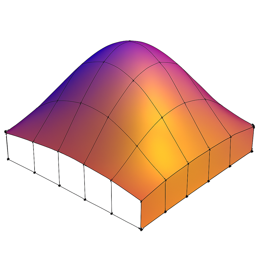
Fig. 99 The final rendering result for 5×5 tessellated mesh.¶ |
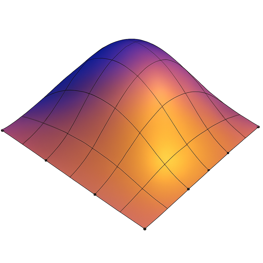
Fig. 100 Geometry Shader (GS) can expand a 5×5 tessellated grid into a 6×6 mesh¶ |
The following TCS glsl from the Red Book can patch high or low resolution of CPs at runtime according the distance of the squre vertices.
Specifying Tessellation Level Factors Using Perimeter Edge Centers.
#version 450 core

// Each patch has four precomputed edge centers:
//   edgeCenter[0] = left edge center
//   edgeCenter[1] = bottom edge center
//   edgeCenter[2] = right edge center
//   edgeCenter[3] = top edge center
struct EdgeCenters {
    vec4 edgeCenter[4];
};

// Array of edge-center data, one entry per patch
uniform EdgeCenters patch[];

// Camera position in world space
uniform vec3 EyePosition;

layout(vertices = 16) out;

void main()
{
    // Pass through control points unchanged
    gl_out[gl_InvocationID].gl_Position =
        gl_in[gl_InvocationID].gl_Position;

    // Synchronize all invocations
    barrier();

    // Only invocation 0 computes tessellation levels
    if (gl_InvocationID == 0)
    {
        // Loop over the four perimeter edges
        for (int i = 0; i < 4; ++i)
        {
            // Distance from eye to this edge center
            float d = distance(
                patch[gl_PrimitiveID].edgeCenter[i],
                vec4(EyePosition, 1.0)
            );

            // Scale factor controlling how quickly tessellation increases
            const float lodScale = 2.5;

            // Convert distance to tessellation level
            float tessLOD = mix(
                0.0,
                gl_MaxTessGenLevel,
                d * lodScale
            );

            gl_TessLevelOuter[i] = tessLOD;
        }
    #if 1
        // Compute the inner tessellation as the average of opposing outer
        // edges: differently from Red Book.
        // It’s what most engines (Unreal, Unity HDRP, Vulkan samples) do.
        // Inner tessellation is the average of outer levels
        float inner = 0.5 *
            (gl_TessLevelOuter[0] + gl_TessLevelOuter[2]);

        inner = clamp(inner, 0.0, gl_MaxTessGenLevel);
        gl_TessLevelInner[0] = inner;
        gl_TessLevelInner[1] = inner;
    #else
        // The Red Book computes outer tessellation levels first, then
        // derives the inner levels from the last computed tessLOD.
        tessLOD = clamp(0.5 * tessLOD, 0.0, gl_MaxTessGenLevel);
        gl_TessLevelInner[0] = tessLOD;
        gl_TessLevelInner[1] = tessLOD;
    #endif
    }
}
The texture function with the argument DisplacementMap in the Red Book, as shown in the following code, does not return color data as in the Fragment Shader. It returns the vertex position data for displacement, such as a roughness map or anything related to surface appearance.
p += texture(DisplacementMap, gl_TessCoord.xy);
Mobile GPU 3D Rendering
The traditional desktop GPUs is IMR — Immediate‑Mode Rendering: Cache misses dominate bandwidth.
TBDR — Tile‑Based Deferred Rendering: Cache misses are nearly eliminated.
Note
Idea:
1. TBDR divides the whole frame into small tiles that fit entirely into on‑chip SRAM.
2. Remove stages of Tessellation Control Shader (TCS), Tessellation Evaluation Shader (TES) and Geometry Shader (GS) since they are optional stages are shown in Fig. 94. Instead, developers use compute shaders before the graphics pipeline to generate meshlets, perform LOD selection, or add extra geometric detail for close‑up room-in effects is shown as Fig. 103.
★ TBDR reduces cache‑miss rate by roughly 10×–50× compared to IMR, because all intermediate color/depth/stencil traffic stays in on‑chip tile memory instead of going to L2/DRAM.
★ Desktop GPUs adopt IMR partly because GS/Tess/Mesh Shaders cannot run efficiently on TBDR. In addition, desktop GPUs adopt IMR because they have the power, bandwidth, and architectural freedom to support unpredictable geometry pipelines and massive workloads that would break TBDR’s tile‑based constraints.
TBDR — Tile‑Based Deferred Rendering
⚠️ For low power mobile device, mobile GPUs use tile-based rendering to reduce the traffice to DRAM as described below:
The traditional desktop GPUs is IMR — Immediate‑Mode Rendering:
IMR: “Draw call arrives → render immediately”
CPU issues DrawCall #1
→ GPU transforms vertices
→ GPU rasterizes fragments
→ GPU writes to DRAM
It never waits to see the rest of the frame.
2. TBDR: “Draw call arrives → store geometry, don’t render yet”. TBDR processes it into two phases as follows:
Phase 1 — Binning (Full‑Frame Geometry Processing) is shown as Fig. 101.
![digraph TBDR_Binning_Flow {
rankdir=LR;
node [shape=box, style=rounded];
CPU_DrawCall [label="CPU Issues Draw Call"];
VS [label="Vertex Shader\n(Transform Vertices)"];
TriangleSetup [label="Triangle Setup\n(Bounding Box, Coverage)"];
Binner [label="Tile Binner\n(Determine Which Tiles Each Triangle Touches)"];
TileLists [label="Per-Tile Triangle Lists\n(Store Geometry, No Rendering Yet)"];
CPU_DrawCall -> VS -> TriangleSetup -> Binner -> TileLists;
}](_images/graphviz-b8ac8ce572f69b89bf0e542dabd73deb1b9cf604.png)
Fig. 101 TBDR Pipeline
When a draw call arrives on a TBDR GPU:
→ It runs the vertex shader
→ It transforms all triangles
→ It determines which tiles each triangle touches
→ It stores triangle references in per‑tile lists is shown as follows:
Example of per‑tile lists
Tile 0 → triangles: [T1, T7, T8, T20]
Tile 1 → triangles: [T2, T3, T7]
Tile 2 → triangles: [T4, T5, T6, T9, T10]
...
Phase 2 — Tile Rendering (Deferred Shading)
For each tile:
→ Load tile’s triangle list
→ Rasterize only those triangles
→ Shade only visible fragments
→ Keep all intermediate buffers in on‑chip SRAM
→ Write final tile to DRAM once
★ As you can see, tile is a small part of rendering frame. In Phase 2 — Tile Rendering, GPU rendering each tile and keep the rendering result of each tile in SRAM.
TBDR Rendering
✅ Rendering flow:
Vertax Shader → Primitive Setup → Tile-Based Culling and Clipping → Rasterization → Fragment Shader
TBDR architectures depend on:
predictable geometry counts,
small on-chip tile memory,
minimal external memory traffic.
⚠️ As described in section 3D Rendering Pipeline, Geometry Shader (GS) can generate both more vertices and more primitives than it receives. A single patch from Tesslation Control Shader (TCS) and Tesslation Evaluation Shader (TVS) can generate millions of micro‑triangles. GS and Tessellation introduce unbounded geometry amplification, which breaks these assumptions and forces expensive DRAM spills for TBDR as shown in Fig. 102,
![digraph TBDR_GS_Comparison {
rankdir=LR;
node [shape=box, style=rounded, fontsize=11];
// Clean TBDR pipeline
subgraph cluster_clean {
label="A. Clean TBDR Pipeline (Mobile GPUs: Mali / PowerVR / Apple)";
style=rounded;
C_VS [label="Vertex Shader\n• Transform\n• Skinning\n• Varyings"];
C_PA [label="Primitive Assembly\n• Triangle setup\n• Culling\n• Clipping"];
C_Tile [label="Tiling / Binning\n• Bin triangles\n• Build tile lists\n• Predictable geometry"];
C_Rast [label="Rasterization\n• Triangle traversal\n• Pixel coverage\n• Early-Z"];
C_FS [label="Fragment Shader\n• Shading\n• Texturing\n• Lighting"];
C_WB [label="Tile Writeback\n• Store tile once\n• Low bandwidth"];
C_VS -> C_PA -> C_Tile -> C_Rast -> C_FS -> C_WB;
}
// GS/Tessellation amplified pipeline
subgraph cluster_gs {
label="B. TBDR with GS/Tessellation (Hypothetical — Why It Breaks)";
style=rounded;
G_VS [label="Vertex Shader"];
G_Tess [label="Tessellation / Geometry Shader\n• 1→64→256 triangles\n• Unbounded amplification\n• View-dependent"];
G_PA [label="Primitive Assembly\n(post-amplification)"];
G_Tile [label="Tiling / Binning\n• Tile list overflow\n• Unpredictable size\n• May spill to DRAM"];
G_Rast [label="Rasterization\n• Heavy load due to amplified geometry"];
G_FS [label="Fragment Shader"];
G_WB [label="Tile Writeback\n• Multiple passes\n• High bandwidth"];
G_VS -> G_Tess -> G_PA -> G_Tile -> G_Rast -> G_FS -> G_WB;
}
// Annotation arrows
G_Tess -> G_Tile [label="massive geometry\namplification", color="red"];
G_Tile -> G_WB [label="DRAM spills\n(high power)", color="red"];
}](_images/graphviz-da0d8487fc2b2189966ed8ee986df42359e8059d.png)
Fig. 102 CPU and GPU Pipeline For Shaders in Mobile Device
This is why Mali, PowerVR, Apple, and Adreno mobile GPUs all omit these stages [41] [42].
Developers manually invoke compute shaders to generate meshlets or additional geometry, adding extra geometric detail for close-up zoom-in effects. Both Mali and PowerVR GPUs then run the standard vertex shader on the generated results.
✔ Step 1 — Developer dispatches a compute shader
This compute shader can do things like:
break a big mesh into meshlets as Fig. 103. The mesh and meshlets are described in the Mesh-Shader Pipeline next section.
generate more vertices for detail (subdivision, displacement)
perform LOD selection
cull invisible meshlets
generate new index/vertex buffers
This is developer‑controlled, not automatic.
![digraph Meshlet_Convert_To_Render_Mobile {
rankdir=LR;
node [shape=box, style=rounded, fontsize=12];
subgraph cluster_input {
label="Input Mesh Data";
style=rounded;
BigMesh [label="Big Mesh\n(Vertex + Index Buffers)"];
}
subgraph cluster_runtime {
label="Runtime / GPU Conversion";
style=rounded;
CS_Convert [label="Compute Shader\n(Convert Mesh → Meshlets,\nCluster Vertices & Triangles,\nCulling, LOD,\nBuild Meshlet Tables)",
style=filled, fillcolor=orange];
Meshlets [label="Generated Meshlets\n(Runtime GPU Data)"];
}
subgraph cluster_render {
label="Mobile Meshlet Rendering Flow\n(Compute + VS Pipeline)";
style=rounded;
VS [label="Mobile Rendering Pipeline\n(VS Pipeline"];
}
BigMesh -> CS_Convert;
CS_Convert -> Meshlets;
Meshlets -> VS;
}](_images/graphviz-dbad710c6206399b37ab311e8caaee4b64156a6a.png)
Fig. 103 CPU and GPU Pipeline For Shader`s in Mobile Device
The compute shader writes results into:
SSBOs
vertex buffers
index buffers
These buffers now contain the final geometry you want to render.
✔ Step 2 — Developer issues a normal draw call
The Mali and PowerVR’s rendering flow is illustrated as Fig. 104.
![digraph Mobile_GPU_Comparison {
rankdir=TB;
node [shape=box, style=rounded, fontsize=11];
// ARM Mali cluster
subgraph cluster_mali {
label="ARM Mali TBDR Pipeline";
style=rounded;
Mali_VS [label="Vertex Shader (VS)\n• Vertex fetch\n• Skinning / morphing\n• Model→World→Clip transforms\n• Varying generation", style="filled,rounded,bold", fillcolor="orange"];
Mali_PA [label="Primitive Assembly\n• Triangle assembly\n• Back-face culling\n• Clipping\n• Viewport transform", style="filled,rounded,bold", fillcolor="lightyellow"];
Mali_Tiling [label="Tiling / Binning\n• Bin triangles into tiles\n• Per-tile visibility\n• Tile list construction"];
Mali_Raster [label="Rasterization\n• Triangle traversal\n• Pixel coverage\n• Early-Z"];
Mali_FS [label="Fragment Shader (FS)\n• Shading\n• Texturing\n• Lighting\n• Blending", style="filled,rounded,bold", fillcolor="orange"];
Mali_Writeback [label="Tile Writeback\n• Store tile to framebuffer\n• Resolve MSAA"];
Mali_VS -> Mali_PA -> Mali_Tiling -> Mali_Raster -> Mali_FS -> Mali_Writeback;
}
// PowerVR cluster
subgraph cluster_powervr {
label="Imagination PowerVR TBDR Pipeline";
style=rounded;
PV_VS [label="Vertex Shader (VS)\n• Vertex fetch\n• Skinning / morphing\n• Transform to clip space\n• Varying generation", style="filled,rounded,bold", fillcolor="orange"];
PV_PB [label="Parameter Buffer (PB)\n• Store transformed vertices\n• Geometry parameter encoding\n• Prepare for tiling", style="filled,rounded,bold", fillcolor="lightyellow"];
PV_Tiling [label="Tiling / Binning\n• Tile list creation\n• Hidden surface removal (HSR)\n• Per-tile visibility"];
PV_Raster [label="Rasterization\n• Triangle traversal\n• Pixel coverage\n• Early-Z"];
PV_FS [label="Fragment Shader (FS)\n• Shading\n• Texturing\n• Lighting\n• Blending", style="filled,rounded,bold", fillcolor="orange"];
PV_Writeback [label="Tile Writeback\n• Store tile to framebuffer\n• Composition"];
PV_VS -> PV_PB -> PV_Tiling -> PV_Raster -> PV_FS -> PV_Writeback;
}
// Compute shader (shared concept)
Compute [shape=box, style="rounded,dashed",
label="Compute Shader (Optional)\n• Culling\n• Skinning\n• Particle simulation\n• Buffer generation\n• Preprocessing"];
CPU [shape=box, style=rounded, label="CPU\n• glDispatchCompute\n• glDraw*"];
// Shared compute flow
CPU -> Compute [label="optional"];
Compute -> Mali_VS [label=<<b><font color="blue">Small Meshlets<br/>in SSBO/buffers</font></b>>];
Compute -> PV_VS [label=<<b><font color="blue">Small Meshlets<br/>in SSBO/buffers</font></b>>];
CPU -> Mali_VS [label="draw call"];
CPU -> PV_VS [label="draw call"];
}](_images/graphviz-ed7695039a41b16216b33ebda721f62661bb2f88.png)
Fig. 104 CPU and GPU Pipeline For Shaders in Mobile Device
Modern mobile engines instead use compute shaders for culling, LOD, meshlet prep, and procedural geometry.
✅ Geometry Shaders are notoriously inefficient even on desktop GPUs. GPU vendors (NVIDIA + AMD + Intel) designed the mesh‑shader pipeline described in the section Mesh-Shader Pipeline.
Mesh-Shader Pipeline
A single 3D object can contain 1 mesh, multiple meshes or hundreds of meshes (complex characters, vehicles, weapons).
Reasons
The purpose of converting a mesh into small clusters (meshlets) is to give the GPU small, coherent, cullable, cache‑friendly work units that dramatically improve parallelism, memory locality, and LOD efficiency.
Raw meshes can have anywhere from thousands to millions of vertices/triangles, while meshlets intentionally restrict clusters to ~32–128 vertices and ~32–256 triangles to maximize GPU efficiency.
Motivation
NVIDIA, AMD, and Intel all needed:
a compute‑like geometry pipeline
meshlet‑based processing
better culling
GPU‑driven rendering
a replacement for VS → TCS → TES → GS
TCS → Fixed-Function Tessellator → TES: geometry amplification.
Fixed‑Function Tessellator: subdivides the patch, generates new domain coordinates and creates the tessellated grid.
Mesh-Shader replaces the fixed‑function tessellator with compute‑like geometry pipeline.
So the vendors co‑designed the hardware pipeline.
✔ Microsoft and Khronos (Vulkan) each standardized it in their own APIs
✅ Solution: As shown in Fig. 105.
![digraph Meshlet_Offline_To_Render {
rankdir=LR;
node [shape=box, style=rounded, fontsize=12];
subgraph cluster_offline {
label="Offline / Build Time";
style=rounded;
BigMesh [label="Big Mesh\n(High-Poly Model)"];
MeshletGen [label="CPU Meshlet Generator Tool\n(Cluster Vertices & Triangles,\nBuild Meshlets, Culling Data)",
style=filled, fillcolor=orange];
Meshlets [label="Small Clusters\n(Meshlets)\n(Precomputed)"];
}
subgraph cluster_runtime {
label="Runtime / Load Time";
style=rounded;
Loader [label="Meshlets Loader\n(Load Meshlet Buffers,\nBuild GPU-Ready Data)"];
}
subgraph cluster_render {
label="Mesh Rendering Flow";
style=rounded;
RenderFlow [label="Mesh Rendering Pipeline\n(Task/Mesh Shader or\nCompute + VS Pipeline)"];
}
BigMesh -> MeshletGen;
MeshletGen -> Meshlets;
Meshlets -> Loader;
Loader -> RenderFlow;
}](_images/graphviz-3f3d973069893eb8e11a9545e824a40362aa658c.png)
Fig. 105 Meshlet Offline To Render
Rendering Pipeline
✔ GPU vendors (NVIDIA + AMD + Intel) designed the mesh‑shader pipeline:
3D Modeling Tool Output (big mesh)
→ CPU Meshlet Generator Tool (offline)
Converting big mesh into small clusters (meshlets) to maximize GPU efficiency.
→ Precomputed meshlets (static clusters)
→ Task Shader (optional)
→ Mesh Shader
3D modeling tools do NOT generate meshlets. Meshlets are always generated later, using specialized meshlet‑generation → tools, most commonly:
NVIDIA meshlet generator (NV_mesh_shader ecosystem)
meshoptimizer (Khronos‑recommended, open source)
Engine‑specific meshlet builders (Unreal, Frostbite, etc.)
So the meshlet conversion happens after the model is exported — not inside Blender, Maya, 3ds Max, etc.
The animation flow from CPU to GPU for Traditional, Compute Shader based and Mesh Shader are shown in Fig. 106, Fig. 107 and Fig. 108.
Mesh shading (Vulkan VK_EXT_mesh_shader, similarly in NV mesh shader) replaces the fixed vertex-input + VS + optional tess/GS stages with a compute-like geometry pipeline:
![digraph CPU_GPU_Pipeline {
rankdir=LR;
node [shape=box, style=rounded, fontsize=12];
subgraph cluster_cpu {
label="CPU";
style=rounded;
CPU_Vertex [label="Load 3D Model\n(Vertex Data)\nVBOs, VAOs, Indices"];
CPU_Anim [label="Update Animation Parameters\n(Bone Matrices, Morph Weights,\nTime, Material Params)"];
}
subgraph cluster_gpu {
label="GPU";
style=rounded;
VS [label="Vertex Shader\n(Skinning, Morphing,\nModel/View/Proj Transform)",
style=filled, fillcolor=orange];
subgraph cluster_optional {
label="Optional Stages";
style="rounded,dashed";
color="gray";
subgraph cluster_ts {
label="Tessellation";
style=rounded;
TCS [label="Tessellation Control Shader\n(TCS)",
style=filled, fillcolor=orange];
TS [label="Fixed-Function Tessellator",
style=filled, fillcolor=orange];
TES [label="Tessellation Evaluation Shader\n(TES)",
style=filled, fillcolor=orange];
TCS -> TS [label="CP + Tessellation level"];
TS -> TES [label="Tessellated domain\ncoordinates"];
{ rank = same; TCS; TS; TES }
}
GS [label="Geometry Shader\n(Primitive Expansion,\nCulling, Layering)",
style=filled, fillcolor=orange];
}
Raster [label="Rasterizer\n(Primitive Assembly,\nClipping, Interpolation)",
style=filled, fillcolor=yellow];
FS [label="Fragment Shader\n(Lighting, Texturing,\nShading, Materials)"];
FB [label="Final Rendered Image\n(Framebuffer Output)"];
}
CPU_Vertex -> VS [label=<<b><font color="red">Big Mesh</font></b>>];
CPU_Anim -> VS;
VS -> TCS [label="Transformed Vertices +\nControl Points(CP)"];
TES -> GS [label="Tessellated Vertices\n(more vertices)"];
GS -> Raster;
Raster -> FS;
FS -> FB;
}](_images/graphviz-001e27daaf1ef8a9d5d084b0ca2b2dbc6f634918.png)
Fig. 106 CPU and GPU Traditional Pipeline For Shaders
![digraph CPU_GPU_MobilePipeline {
rankdir=LR;
node [shape=box, style=rounded, fontsize=12];
subgraph cluster_cpu {
label="CPU";
style=rounded;
CPU_Vertex [label="Load 3D Model\n(Vertex Data)\nVBOs, VAOs, Indices"];
CPU_Anim [label="Update Animation Parameters\n(Bone Matrices, Morph Weights,\nTime, Material Params)"];
}
subgraph cluster_gpu {
label="GPU (Mobile / TBDR)";
style=rounded;
CS_Meshlet [label="Compute Shader\n(Generate Meshlets,\nCulling, LOD,\nBuild Indirect Draw Cmds)",
style=filled, fillcolor=orange];
VS [label="Vertex Shader\n(Transform, Skinning,\nMorphing, MVP)"];
Raster [label="Rasterizer\n(Primitive Assembly,\nClipping, Interpolation)",
style=filled, fillcolor=yellow];
FS [label="Fragment Shader\n(Lighting, Texturing,\nShading, Materials)"];
FB [label="Final Rendered Image\n(Framebuffer Output)"];
}
CPU_Vertex -> CS_Meshlet;
CPU_Anim -> CS_Meshlet;
CS_Meshlet -> VS [label=<<b><font color="blue">Small Meshlets</font></b>>];
VS -> Raster;
Raster -> FS;
FS -> FB;
}](_images/graphviz-ba7ee75e7abec13829d22c7a2bcc2f7b8fb9fb44.png)
Fig. 107 CPU and GPU Mobile Pipeline For Shaders
![digraph CPU_GPU_Pipeline {
rankdir=LR;
node [shape=box, style=rounded, fontsize=12];
subgraph cluster_cpu {
label="CPU";
style=rounded;
CPU_Vertex [label="Load 3D Model\n(Vertex Data)\nVBOs, VAOs, Indices"];
MeshletGen [label="Meshlet Generator Tool\n(Cluster Vertices & Triangles,\nBuild Meshlets, Culling Data)", style=filled, fillcolor=orange];
CPU_Anim [label="Update Animation Parameters\n(Bone Matrices, Morph Weights,\nTime, Material Params)"];
}
subgraph cluster_gpu {
label="GPU";
style=rounded;
TaskS [label="Task Shader (Optional)\n(Work Distribution,\nMeshlet Dispatch)", style=filled, fillcolor=orange];
MeshS [label="Mesh Shader\n(Expand Meshlets,\nCulling, LOD,\nEmit Triangles\nskinning)", style=filled, fillcolor=orange];
Raster [label="Rasterizer\n(Consumes Mesh Shader Output,\nClipping, Interpolation)", style=filled, fillcolor=yellow];
FS [label="Fragment Shader\n(Lighting, Texturing,\nShading, Materials)"];
FB [label="Final Rendered Image\n(Framebuffer Output)"];
}
CPU_Vertex -> MeshletGen;
MeshletGen -> TaskS [label=<<b><font color="blue">Small Meshlets</font></b>>];
CPU_Anim -> TaskS;
TaskS -> MeshS;
MeshS -> Raster;
Raster -> FS;
FS -> FB;
}](_images/graphviz-e51f607f338d5730208764bc92221d573274c56c.png)
Fig. 108 CPU and GPU Mesh Shader Pipeline For Shaders
As in Fig. 108, NVIDIA/AMD desktop provide mesh‑shader to do the following pipeline.
Task Shader Responsibilities
The Task Shader acts as a coarse-grained work distributor.
Key responsibilities:
Perform coarse culling at the meshlet or instance level.
Select appropriate LODs for distant geometry.
But it does not create new detail like the Tessellation Shaders.
Build a compact list of meshlets to be processed.
Determine how many mesh shader workgroups to launch.
Pass a payload (task data) to mesh shader workgroups.
The task shader does not emit vertices or primitives.
Mesh Shader Responsibilities
The mesh shader replaces the vertex shader, tessellation, and often the geometry shader. It operates on meshlets inside workgroups.
Key responsibilities:
Load meshlet vertices and indices from GPU memory.
Apply transforms, skinning, morphing, and procedural deformation.
Mesh Shader outputs exactly what the meshlet contains usually, unless you code it manually.
Custom procedural code inside a Mesh Shader can generate more vertices, subdivide triangles, procedurally generate detail, amplify geometry. Mesh Shaders replace Vertex Shader, Geometry Shader and Tessellation (optional). But they do not perform automatic tessellation. They simply take a meshlet, run a workgroup and output the triangles inside that meshlet.
Perform fine-grained culling: - frustum culling - backface culling - small triangle culling - cluster-level culling
Generate the final set of vertices and primitives.
Emit primitives directly to the rasterizer.
Because mesh shaders run in workgroups, they can use shared memory and synchronize threads, enabling efficient reuse of vertex data.
Why Meshlets Fit GPU Architecture Well
Meshlets align naturally with GPU hardware for several reasons:
Workgroup-Friendly: Each meshlet maps cleanly to a single workgroup, keeping memory usage predictable and minimizing divergence.
Cache Efficiency: Meshlets maximize vertex reuse and reduce memory bandwidth by grouping spatially local geometry.
Hierarchical Culling: - Task shader: coarse culling of entire meshlets. - Mesh shader: fine culling of individual primitives.
Reduced CPU Overhead: The GPU can perform culling, LOD selection, and primitive generation without CPU intervention, enabling GPU-driven rendering.
Scalable Parallelism: Each meshlet is processed independently, allowing thousands of workgroups to run in parallel across GPU SMs.
Both Mobile GPU and Mesh-Shader GPU convert big mesh to small meshlets and render them efficiently using GPU SIMT executation and memory hierarchy. The comparsion is shown in the following table.
Comparsion: Mobile GPU (Compute-Shader Based) vs Desktop Mesh-Shader GPU
The Mesh Shader is similar to the previous section of Mobile Compute Shader based Meshlets as the following table:
Concept |
Mobile GPU (Compute-Shader Based) |
Desktop Mesh-Shader GPU |
|---|---|---|
Meshlet generation |
Compute Shader generates meshlets at runtime |
CPU Meshlet Generator Tool (offline) |
Tile-based |
Yes |
No |
Work distribution |
Compute Shader dispatch groups handle distribution |
Task Shader distributes meshlet workloads |
Meshlet expansion |
Vertex Shader processes vertices after compute pre-processing |
Mesh Shader expands meshlets and emits triangles |
Culling & LOD |
Compute Shader performs culling and LOD before raster |
Task + Mesh Shader perform culling and LOD selection |
Draw submission |
Compute Shader writes indirect draw commands |
Mesh Shader emits primitives directly to rasterizer |
Pipeline family |
Traditional Pipeline (VS → Raster → FS) |
Mesh-Shader Pipeline (Task → Mesh → Raster → FS) |
Summary
Meshlets and the mesh-shader pipeline transform geometry processing into a compute-like workflow. By organizing geometry into small, cache-friendly clusters and distributing work across task and mesh shaders, modern GPUs achieve higher throughput, better culling efficiency, and reduced CPU overhead compared to the traditional vertex-processing pipeline.
Animation Example
The skinning formula is described in SW Stack and Data Flow section as follows:
The following code implements the formula shown above.
GLSL Vertex Shader
layout(location = 0) in vec3 position;
layout(location = 1) in uvec4 boneIndex;
layout(location = 2) in vec4 boneWeights;

// Simple Uniforms (non-UBO)
uniform mat4 boneMatrices[100];
uniform mat4 model;
uniform mat4 view;
uniform mat4 projection;

vec4 skinnedPos = vec4(0.0);
for (int i = 0; i < 4; ++i) {
    skinnedPos += boneMatrices[boneIndex[i]] * vec4(position, 1.0) * boneWeight[i];
}
gl_Position = projection * view * model * skinnedPos;
Here:
position, boneIndex, boneWeight = vertex attributes
boneMatrices, model, view, projection = uniforms
The OpenGL code used to pass these varaibles to GLSL will be shown in OpenGL API Commands That Trigger GPU Skinning later. The OpenGL API sets position, boneIndex and boneWeight to locations 0, 1 and 2, respectively, using glVertexAttribPointer.
void glVertexAttribPointer(GLuint index, GLint size, GLenum type, GLboolean normalized, GLsizei stride, const GLvoid * pointer);
Examples:
glBindBuffer(GL_ARRAY_BUFFER, vboPositions);
glVertexAttribPointer(0, 3, GL_FLOAT, GL_FALSE, stride, offset); → layout(location = 0) in vec3 position;
glBindBuffer(GL_ARRAY_BUFFER, vboBoneIndex);
glVertexAttribIPointer(1, 4, GL_UNSIGNED_BYTE, stride, offset); → layout(location = 1) in uvec4 boneIndex;
Bone indices are small integers (0–255), so storing them as GL_UNSIGNED_BYTE: OpenGL will automatically zero‑extend 8‑bit unsigned integers into 32‑bit unsigned integers inside the shader.
✔ Why boneIndex[] and boneWeight[] are 3D Model Information
These two arrays describe how the mesh is bound to the skeleton.
They are part of the static mesh data, created during rigging in Blender/Maya/etc.
boneIndex[] → tells which bone
For each vertex: which bones influence it
Example: { 3, 7, 12, 0 }
boneWeight[] → tells how much
For each vertex: how much each bone influences it
Example: { 0.5, 0.3, 0.2, 0.0 }
These values never change during animation. They are baked into the mesh and stored in the VBO as vertex attributes.
✔ Why boneMatrices[] is Animation Parameters
boneMatrices[] → tells where the bone is this frame
Example: boneMatrices[3] (upper arm bone this frame)
[ 0.87 -0.49 0.00 0.12 ] [ 0.49 0.87 0.00 0.03 ] [ 0.00 0.00 1.00 0.00 ] [ 0.00 0.00 0.00 1.00 ]
This matrix might represent:
a 30° rotation of the upper arm
plus a small translation (0.12, 0.03, 0.0)
Animation Parameters are dynamic per‑frame data, such as:
bone matrices
animation time
morph weights
blend factors
procedural animation inputs
These change every frame.
✔ OpenGL API Commands That Trigger GPU Skinning
Overview
In OpenGL, animation is not built into the API. Instead, animation occurs because the application updates Animation Parameters (such as bone matrices) and the vertex shader interprets them. The GPU performs the animation math during the draw call.
The following sections describe the exact OpenGL commands involved in triggering GPU-based vertex animation.
Updating Animation Parameters (Uniforms or UBOs)
Animation Parameters such as boneMatrices[] are updated every frame.
They are supplied to the vertex shader as uniforms or through a uniform
buffer object (UBO).
Uniform array example:
// Matrix Uniforms
GLint locModel = glGetUniformLocation(program, "model");
GLint locView  = glGetUniformLocation(program, "view");
GLint locProj  = glGetUniformLocation(program, "proj");

glUniformMatrix4fv(locModel, 1, GL_FALSE, glm::value_ptr(modelMatrix));
glUniformMatrix4fv(locView,  1, GL_FALSE, glm::value_ptr(viewMatrix));
glUniformMatrix4fv(locProj,  1, GL_FALSE, glm::value_ptr(projMatrix));

// Bone Matrix Array
GLint loc = glGetUniformLocation(program, "boneMatrices");
glUniformMatrix4fv(loc, boneCount, GL_FALSE, boneMatrixData);
Uniform Buffer Object example:
glBindBuffer(GL_UNIFORM_BUFFER, boneUBO);
glBufferSubData(GL_UNIFORM_BUFFER, 0, size, boneMatrixData);
glBindBufferBase(GL_UNIFORM_BUFFER, bindingPoint, boneUBO);
These commands send the per-frame animation data to the GPU.
Binding Vertex Data (Mesh Information)
Static mesh data such as positions, normals, boneIndex[] and
boneWeight[] is stored in vertex buffer objects (VBOs) and attached
to a vertex array object (VAO).
glBindVertexArray(vao);

glBindBuffer(GL_ARRAY_BUFFER, vboPositions);
glVertexAttribPointer(0, 3, GL_FLOAT, GL_FALSE, stride, offset);

// Activate attribute location 1, then ehe shader’s layout(location = 1)
// input receives real data.
glEnableVertexAttribArray(0);

glBindBuffer(GL_ARRAY_BUFFER, vboBoneIndex);
glVertexAttribIPointer(1, 4, GL_UNSIGNED_BYTE, stride, offset);
glEnableVertexAttribArray(1);

glBindBuffer(GL_ARRAY_BUFFER, vboBoneWeight);
glVertexAttribPointer(2, 4, GL_FLOAT, GL_FALSE, stride, offset);
glEnableVertexAttribArray(2);
These commands provide the static 3D model information to the vertex shader.
Activating the Shader Program
The vertex shader containing the skinning logic must be activated before drawing.
glUseProgram(program);
This step ensures that the GPU will execute the correct vertex shader when the draw call is issued.
Issuing the Draw Call (Animation Trigger)
The draw call is the moment when the GPU executes the vertex shader for each vertex. This is where animation actually happens.
glDrawElements(GL_TRIANGLES, indexCount, GL_UNSIGNED_INT, 0);
or:
glDrawArrays(GL_TRIANGLES, 0, vertexCount);
The vertex shader runs once per vertex, combining:
vertex attributes (
position,boneIndex[],boneWeight[])animation parameters (
boneMatrices[])
to compute the animated vertex position.
Summary Table
Purpose |
Data Type |
OpenGL API |
Static or Dynamic |
|---|---|---|---|
Mesh data (positions, bone indices, bone weights) |
Vertex Attributes |
|
Static (stored in VBO) |
Animation Parameters (bone matrices) |
Uniforms / UBO |
|
Dynamic (updated every frame) |
Activate shader program |
Shader Program |
|
Per draw |
Trigger animation |
Draw Call |
|
Per frame |
Conclusion
OpenGL does not provide a built-in animation system. Instead, animation occurs because the application updates Animation Parameters each frame and the vertex shader applies animation math during the draw call. The GPU performs the animation only when the draw command is issued.
GLSL (GL Shader Language)
OpenGL is a standard specification for designing 2D and 3D graphics and animation in computer graphics. To support advanced animation and rendering, OpenGL provides a large set of APIs (functions) for graphics processing. Popular 3D modeling and animation tools—such as Maya, Blender, and others—can utilize these APIs to handle 3D-to-2D projection and rendering directly on the computer.
The hardware-specific implementation of these APIs is provided by GPU manufacturers, ensuring that rendering is optimized for the underlying hardware.
Background
In the previous section SW Stack and Data Flow described how each frame is generated to display the movement animation or skinning effects using the small animation parameters stored in 3D model and sent from CPU.
Based on description of section SW Stack and Data Flow, we know the animation can be implemented using fixed‑function skinning. The following are the animation examples for shader-less era.
✔ Some consoles and mobile GPUs did have fixed‑function skinning.
✔ In those systems, you could upload bone matrices and let hardware animate vertices.
❌ But you could not change the formulas — only use the built‑in ones.
The following console GPUs did have fixed‑function skinning:
PlayStation 2 (PS2) — VU0/VU1 Microcode
PS2 had fixed hardware instructions for:
skinning
morphing
matrix blending
Developers could upload bone matrices and let the hardware do the blending. No shaders existed yet.
Nintendo GameCube / Wii — XF Unit
The GameCube GPU had a fixed‑function transform unit that supported:
matrix palette skinning (up to 10 matrices)
per‑vertex weighted blending
Again, no shaders — but hardware skinning existed.
The previous section Role and Purpose of Shaders also explained different visual effects can be achieved by switching shaders to shapplying different materials across frames.
❌ However the fixed‑function pipeline (OpenGL 1.x / early 2.x without shaders) has:
no per‑vertex programmable math
no access to bone matrices
no ability to blend multiple positions
no ability to apply time‑based deformation
no ability to read custom vertex attributes
no ability to modify vertex positions except via the model‑view matrix
❌ As result the shader-less (fixed-function) pipeline in early OpenGL did not support GPU-based skinning. Skinning had to be implemented on the CPU, which imposed limitations on both animation capability and performance, as described below:
Major Disadvantages of a Shader-less (Fixed-Function) Pipeline
No GPU-side animation
Cannot perform skinning, morphing, or procedural deformation on the GPU.
All animation must be computed on the CPU, causing performance bottlenecks.
Limited lighting and materials
Only fixed-function lighting is available.
No custom BRDFs, PBR workflows, toon shading, or stylized effects.
No procedural or time-based effects
Cannot implement UV animation, distortion, dissolve, holograms, or particle effects.
No access to noise functions or time-driven logic in the pipeline.
No post-processing
Motion blur, bloom, depth of field, color grading, and screen-space effects are impossible.
Rigid data flow
Cannot define custom vertex attributes, varyings, or uniform buffers.
Material and animation systems cannot be data-driven.
Poor scalability and performance
CPU must update all animated geometry every frame.
GPU parallelism is unused, limiting scene complexity.
Deprecated and non-portable
Fixed-function pipeline is removed in modern OpenGL core profiles.
Not compatible with contemporary engines or hardware.
✔ All modern consoles (PS5, PS5 Pro, PS6‑class hardware of Sony, Switch 2 of Nintendo) use programmable shader architectures rather than fixed‑function animation hardware. Fixed-function animation is now obsolete.
Sony’s current and upcoming GPUs are based on AMD RDNA architectures, which are fully programmable shader GPUs.
Nintendo’s upcoming Switch 2 uses a custom Nvidia Ampere GPU.
Examples
An OpenGL program typically follows a structure like the example below:
Vertex shader
#version 330 core
layout (location = 0) in vec3 aPos; // the position variable has attribute position 0

out vec4 vertexColor; // specify a color output to the fragment shader

void main()
{
    gl_Position = vec4(aPos, 1.0); // see how we directly give a vec3 to vec4's constructor
    vertexColor = vec4(0.5, 0.0, 0.0, 1.0); // set the output variable to a dark-red color
}
Fragment shader
#version 330 core
out vec4 FragColor;

in vec4 vertexColor; // the input variable from the vertex shader (same name and same type)

void main()
{
    FragColor = computeColorOfThisPixel(...);
}
OpenGL user program
int main(int argc, char ** argv)
{
  // init window, detect user input and do corresponding animation by calling opengl api
  ...
}
The last main() function in an OpenGL application is written by the user, as expected. Now, let’s explain the purpose of the first two main components of the OpenGL pipeline.
As discussed in the Concepts of Computer Graphics textbook, OpenGL provides a rich set of APIs that allow programmers to render 3D objects onto a 2D computer screen. The general rendering process follows these steps:
The user sets up lighting, textures, and object materials.
The system calculates the position of each vertex in 3D space.
The GPU and rendering pipeline automatically determine the color of each pixel based on lighting, textures, and interpolation.
The final image is displayed on the screen by writing pixel colors to the framebuffer.
To give programmers the flexibility to add custom effects or visual enhancements—such as modifying vertex positions for animation or applying unique coloring—OpenGL provides two programmable stages in the graphics pipeline:
Vertex Shader: Allows the user to customize how vertex coordinates are transformed and processed.
Fragment Shader: Allows the user to define how each pixel (fragment) is shaded and colored, enabling effects like lighting, textures, and transparency.
These shaders are written by the user and compiled at runtime, providing powerful control over the rendering process.
OpenGL uses fragment shader instead of pixel is : “Fragment shaders are a more accurate name for the same functionality as Pixel shaders. They aren’t pixels yet, since the output still has to past several tests (depth, alpha, stencil) as well as the fact that one may be using antialiasing, which renders one-fragment-to-one-pixel non-true [55]. Programmer is allowed to add their converting functions that compiler translate them into GPU instructions running on GPU processor. With these two shaders, new features have been added to allow for increased flexibility in the rendering pipeline at the vertex and fragment level [56]. Unlike the shaders example here [57], some converting functions for coordinate in vertex shader or for color in fragment shade are more complicated according the scenes of animation. Here is an example [58]. In wiki shading page [3], Gourand and Phong shading methods make the surface of object more smooth by glsl. Example glsl code of Gourand and Phong shading on OpenGL api are here [59]. Since the hardware of graphic card and software graphic driver can be replaced, the compiler is run on-line meaning driver will compile the shaders program when it is run at first time and kept in cache after compilation [60].
The shaders program is C-like syntax and can be compiled in few mini-seconds, add up this few mini-seconds of on-line compilation time in running OpenGL program is a good choice for dealing the cases of driver software or gpu hardware replacement [61].
Goals
Goals of GLSL Shader Language:
GLSL was designed for real-time graphics using programmable GPUs.
Programmable Pipeline:
Custom control over vertex, fragment, and other pipeline stages
Enables dynamic effects, lighting, animation, and transformations
GPU Acceleration
Executes on GPU cores for massive parallel performance
Optimized for matrix and vector operations common in graphics
Cross-Platform Compatibility:
Runs consistently across OSes and hardware via OpenGL
Avoids vendor lock-in for portable shader code
C-Like Syntax
Familiar syntax for developers used to C-style languages
Supports functions, loops, conditionals, and custom types
Fine-Grained Rendering Control
Direct access to geometry, color, texture, lighting parameters
Enables advanced effects like shadows, fog, reflections
Real-Time Interactivity
Responds to user input, time, and animations at runtime
Suitable for games, simulations, and creative tools
Minimal Host Dependency
Executes within the graphics driver context
No need for external libraries, file I/O, or system calls
GLSL vs. C: Feature Overview
GLSL expands upon C for GPU-based graphics programming.
Additions to C:
Specialized Data Types
vec2, vec3, vec4: float vectors
mat2, mat3, mat4: float matrices
bvec, ivec, uvec, dvec: boolean and integer vectors
sampler2D, samplerCube: texture samplers
Pipeline Qualifiers
attribute, varying (legacy)
in, out, inout: stage and parameter I/O
uniform: uniform variables are set externally by the host application (e.g., OpenGL) and remain constant across all shader invocations for a draw call.
layout(location = x): set GPU variable locations. See Animation Example section.
precision qualifiers: lowp, mediump, highp
Built-in Functions
texture(), reflect(), refract(), normalize()
mix(), smoothstep(): interpolation and blending
dot(), cross(), transpose(), inverse(): math ops
dFdx(), dFdy(), fwidth(): pixel derivatives
Swizzling
.xyzw, .rgba, .stpq access vector components
e.g., vec4 pos = vec3(1, 2, 3).xyzx
Shader-Specific Keywords
discard: drop fragments early
gl_Position, gl_FragColor, gl_VertexID: built-ins
subroutine, patch, sample: advanced pipeline control
Removals and Restrictions:
No Pointers or Memory Access
No * or & operators
No malloc, free
No File I/O or Standard C Libs
No stdio.h, printf(), fopen()
No Recursion
Recursive functions not allowed
No #include Support
Files can’t be included via preprocessor
Limited Control Flow
goto not allowed
Loops must be statically determinable in many cases for compiler optimization as follows:
Example for loops must be statically determinable in many cases
const int MAX_LIGHTS = 10;
for (int i = 0; i < MAX_LIGHTS; ++i) {
  // Safe: MAX_LIGHTS is a compile-time constant
}
Restricted C Keywords
typedef, union, enum, class, namespace, inline, etc.
Reserved or disallowed
Notes:
Changes help GPU execute safely in parallel
Designed for real-time, interactive graphics
GLSL Qualifiers by Shader Stage
The CPU and GPU Pipeline For Shaders is introduced in section 3D Rendering Pipeline. The Fig. 109 is the summary of GLSL Qualifiers below.
![digraph CPU_GPU_Pipeline {
rankdir=LR;
node [shape=box, style=rounded, fontsize=12];
subgraph cluster_cpu {
label="CPU";
style=rounded;
CPU_Vertex [label="Load 3D Model\n(Per-Vertex Attributes)\nVBOs, VAOs, Indices"];
CPU_Anim [label="Uniform Updates\n(Animation Parameters,\nMatrices, Lighting,\nMaterial Params)"];
}
subgraph cluster_gpu {
label="GPU";
style=rounded;
VS [label="Vertex Shader\nInputs:\n - Vertex Attributes (in)\n - Uniforms (matrices, animation)\nOutputs:\n - Varyings → Rasterizer"];
Raster [label="Rasterizer\n(Primitive Assembly,\nClipping, Interpolation)\nOutputs:\n - Interpolated Varyings"];
FS [label="Fragment Shader\nInputs:\n - Interpolated Data (in)\n - Uniforms (textures, lighting)\nOutputs:\n - Final Fragment Color"];
FB [label="Framebuffer\n(Final Rendered Image)"];
CS [label="Compute Shader\n(Workgroups, SSBOs,\nImages, Shared Memory)\nIndependent of VS→FS Pipeline"];
}
# Main graphics pipeline
CPU_Vertex -> VS;
CPU_Anim -> VS;
VS -> Raster;
Raster -> FS;
FS -> FB;
# Compute shader is dispatched separately
CPU_Anim -> CS [style=dashed, label="Dispatch Compute"];
}](_images/graphviz-e2594ff1194a5682c90bb59fc5a1d7670c5b8b27.png)
Fig. 109 Shaders input and output
Vertex Shader:
in: Receives per-vertex attributes from buffer objects, it is 3D Model Information described in Fig. 109.
out: Passes data to next stage (e.g., fragment shader)
uniform: Global parameters like matrices or lighting, it is Animation Parameters, also referred to as Uniform Updates described in Fig. 109. The Animation Example section provides an example in Vertex Shader (VS) that demostrates animation using both the 3D model information and Uniform Updates.
layout(location = x): Binds input/output to attribute index. See Animation Example section.
const: Compile-time constants
Cannot use interpolation qualifiers on inputs
Fragment Shader:
in: Receives interpolated data from previous stage as shown in Fig. 109.
out: Writes Final Fragement Color to FrameBuffer
uniform: Global parameters like textures or lighting as shown in Fig. 109. Uniform data remains unchanged across all pipeline stages and is shared by all shaders in the pipeline. This means that uniform data represents global parameters for 3D GPU rendering.
flat: Disables interpolation; uses provoking vertex
smooth: Enables perspective-correct interpolation (default)
noperspective: Linear interpolation in screen space
centroid: Samples within primitive area (for multisampling)
sample: Per-sample interpolation (GLSL 4.0+)
discard: Terminates fragment processing early
Compute Shader:
layout(local_size_x = x): Defines workgroup size
uniform: Input parameters from host
buffer: Shader storage buffer access
shared: Shared memory among invocations in a workgroup
image2D, image3D: Direct image access
coherent, volatile, restrict: Memory access control
readonly, writeonly: Access mode for image/buffer
Compute shader: may be applied in any stage as described in section 3D Rendering Pipeline.
Common Across Stages:
const: Immutable values
uniform: Host-set global parameters
layout(binding = x): Bind uniform/buffer/image to index
precise: Ensures consistent computation
invariant: Prevents variation across shader executions
Notes:
attribute and varying are deprecated (use in/out instead)
Interpolation qualifiers only affect fragment shader inputs
Uniforms are shared across all stages and remain constant
Examples of GLSL Qualifiers by Shader Stage
// ==============================================
// Vertex Shader: Qualifier Summary (GLSL)
// ==============================================

// Vertex inputs
layout(location = 0) in vec3 aPosition;   // in: per-vertex attribute
layout(location = 1) in vec3 aNormal;

// Outputs to fragment shader
out vec3 vNormal;                         // out: passes to next stage

// Uniforms
uniform mat4 uModelMatrix;               // uniform: global parameter
uniform mat4 uViewProjectionMatrix;

// Constants
const float PI = 3.14159265;             // const: compile-time constant

void main() {
  vNormal = aNormal;
  gl_Position = uViewProjectionMatrix * uModelMatrix * vec4(aPosition, 1.0);
}

// ==============================================
// Fragment Shader: Qualifier Summary (GLSL)
// ==============================================

// Inputs from vertex shader
in vec3 vNormal;                          // in: interpolated input

// Output to framebuffer
out vec4 fragColor;                       // out: final pixel color

// Uniforms
uniform vec3 uLightDirection;            // uniform: shared global input
uniform vec3 uBaseColor;

// Interpolation control
// flat in vec3 vFlatColor;              // flat: no interpolation
// smooth in vec3 vSmoothColor;         // smooth: default interpolation
// noperspective in vec3 vLinearColor;  // noperspective: screen-space linear

void main() {
  float brightness = max(dot(normalize(vNormal), uLightDirection), 0.0);
  fragColor = vec4(uBaseColor * brightness, 1.0);
}

// ==============================================
// Compute Shader: Qualifier Summary (GLSL)
// ==============================================

#version 430

// Workgroup size
layout(local_size_x = 16, local_size_y = 16) in;

// Shared memory
shared float tileData[256];              // shared: intra-group memory

// Uniforms
uniform float uTime;                     // uniform: global input

// Buffer access
layout(std430, binding = 0) buffer DataBuffer {
  float values[];
};

// Image access
layout(binding = 1, rgba32f) uniform image2D uImage;

// Memory qualifiers
// coherent, volatile, restrict, readonly, writeonly

void main() {
  uint idx = gl_GlobalInvocationID.x;
  values[idx] += sin(uTime);           // buffer write
  imageStore(uImage, ivec2(idx, 0), vec4(values[idx])); // image write
}
OpenGL Shader Compiler
The OpenGL standard is defined in [62]. OpenGL is primarily designed for desktop computers and servers, whereas OpenGL ES is a subset tailored for embedded systems [63].
Although shaders represent only a small part of the entire OpenGL software/hardware stack, implementing a compiler for them is still a significant undertaking. This is because a large number of APIs need to be supported. For instance, there are over 80 texture-related APIs alone [64].
A practical approach to implementing such a compiler involves generating LLVM extended intrinsic functions from the shader frontend (parser and AST generator). These intrinsics can then be lowered into GPU-specific instructions in the LLVM backend. The overall workflow is illustrated as follows:
Fragment shader
#version 320 es
uniform sampler2D x;
out vec4 FragColor;

void main()
{
    FragColor = texture(x, uv_2d, bias);
}
llvm-ir
...
!1 = !{!"sampler_2d"}
!2 = !{i32 SAMPLER_2D} ; SAMPLER_2D is integer value for sampler2D, for example: 0x0f02
; A named metadata.
!x_meta = !{!1, !2}

define void @main() #0 {
    ...
    %1 = @llvm.gpu0.texture(metadata !x_meta, %1, %2, %3); ; %1: %sampler_2d, %2: %uv_2d, %3: %bias
    ...
}
asm of gpu
...
// gpu machine code
load $1, tex_a;
sample2d_inst $1, $2, $3 // $1: tex_a, $2: %uv_2d, $3: %bias

.tex_a // Driver set the index of gpu descriptor regsters here
As shown at the end of the code above, the .tex_a memory address contains the Texture Object, which is bound by the driver during online compilation and linking. By binding a Texture Object (software representation) to a Texture Unit (hardware resource) via OpenGL API calls, the GPU can access and utilize Texture Unit hardware efficiently. This binding mechanism ensures that texture sampling and mapping are executed with minimal overhead during rendering.
For more information about LLVM extended intrinsic functions, please refer to [65].
gvec4 texture(gsampler2D sampler, vec2 P, [float bias]);
GPUs provide Texture Units to accelerate texture access in fragment shaders. However, Texture Units are expensive hardware resources, and only a limited number are available on a GPU. To manage this limitation, the OpenGL driver can associate a Texture Unit with a sampler variable using OpenGL API calls. This association can be updated or switched between shaders as needed. The following statements demonstrate how to bind and switch Texture Units across shaders:
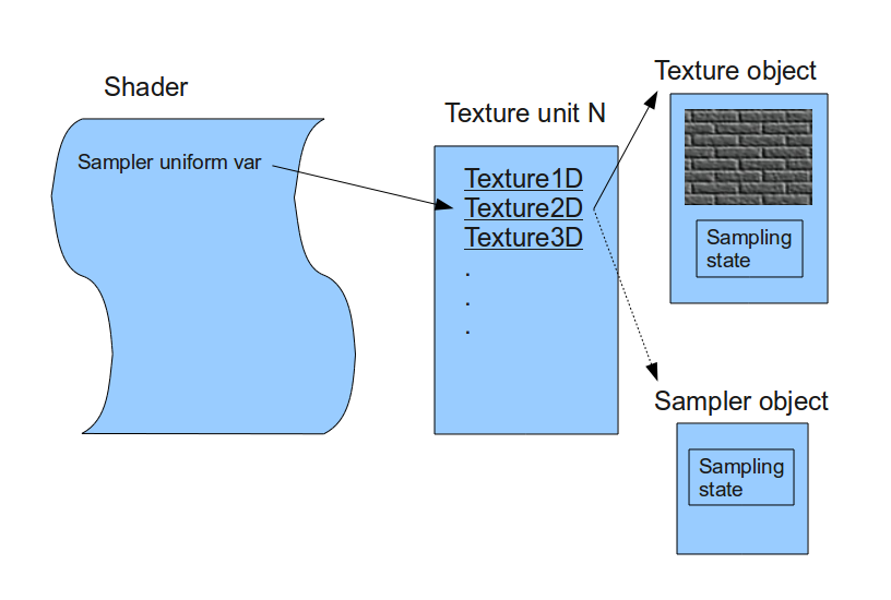
As shown in Fig. 110, the texture object is not bound directly to a shader (where sampling operations occur). Instead, it is bound to a texture unit, and the index of this texture unit is passed to the shader. This means the shader accesses the texture object through the assigned texture unit. Most GPUs support multiple texture units, though the exact number depends on the hardware capabilities [66].
A texture unit—also known as a Texture Mapping Unit (TMU) or Texture Processing Unit (TPU)— is a dedicated hardware component in the GPU that performs texture sampling operations.
The sampler argument in the texture sampling function refers to a sampler2D (or similar) uniform variable. This variable represents the texture unit index used to access the associated texture object [66].
Sampler Uniform Variables:
OpenGL provides a set of special uniform variables for texture sampling, named according to the texture target: sampler1D, sampler2D, sampler3D, samplerCube, etc.
You can create as many sampler uniform variables as needed and assign each one to a specific texture unit index using OpenGL API calls. Whenever a sampling function is invoked with a sampler uniform, the GPU uses the texture unit (and its bound texture object) associated with that sampler [66].
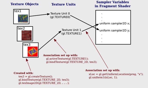
For Java programmers, JOGL provides same level of API in Java for wrapping to OpenGL C API. As shown in Fig. 111, the JOGL gl.bindTexture() binds a Texture Object to a specific Texture Unit. Then, using gl.getUniformLocation() and gl.uniform1i(), you associate the Texture Unit with a sampler uniform variable in the shader.
For example, gl.uniform1i(xLoc, 1) assigns Texture Unit 1 to the sampler variable at location xLoc. Similarly, passing 2 would refer to Texture Unit 2, and so on [67].
The following Fig. 112 illustrates how the OpenGL driver reads metadata from a compiled GLSL object, how the OpenGL API links sampler uniform variables to Texture Units, and how the GPU executes the corresponding texture instructions.
![digraph G {
graph [rankdir=TB];
// ---------------------
// Node n1, n2, n3, n4
// ---------------------
n1 [shape=box, label="1. GPU Compiler"];
n2 [shape=box, label="2. Driver alloc memory xLoc for x"];
n3 [shape=box, label="3. xLoc = gl.getUniformLocation(prog, \"x\")"];
n4 [shape=box, label="4. gl.uniform1i(xLoc, 1)"];
// -------------------------
// Table 1 (tbl1)
// -------------------------
tbl1 [
shape=none
label=<
<TABLE BORDER="1" CELLBORDER="1" CELLSPACING="0">
<TR><TD COLSPAN="3"><B>driver Sampler Variables table</B></TD></TR>
<TR>
<TD PORT="r0c0">name</TD>
<TD PORT="r0c1">type</TD>
<TD PORT="r0c2">location</TD>
</TR>
<TR>
<TD PORT="r1c0">...</TD>
<TD PORT="r1c1"></TD>
<TD PORT="r1c2"></TD>
</TR>
<TR>
<TD PORT="r2c0">"x"</TD>
<TD PORT="r2c1">SAMPLE_2D</TD>
<TD PORT="r2c2">xLoc</TD>
</TR>
<TR>
<TD PORT="r3c0">...</TD>
<TD PORT="r3c1"></TD>
<TD PORT="r3c2"></TD>
</TR>
</TABLE>
>
];
// -------------------------
// Table 2 (tbl2)
// -------------------------
tbl2 [
shape=none
label=<
<TABLE BORDER="1" CELLBORDER="1" CELLSPACING="0">
<TR><TD COLSPAN="4"><B>texture descriptor</B></TD></TR>
<TR>
<TD PORT="t0c0">offset</TD>
<TD PORT="t0c1">location</TD>
<TD PORT="t0c2">Texture Unit</TD>
</TR>
<TR>
<TD PORT="t1c0">...</TD>
<TD PORT="t1c1"></TD>
<TD PORT="t1c2"></TD>
</TR>
<TR>
<TD PORT="t2c0">k</TD>
<TD PORT="t2c1">xLoc</TD>
<TD PORT="t2c2">1</TD>
</TR>
<TR>
<TD PORT="t3c0">...</TD>
<TD PORT="t3c1"></TD>
<TD PORT="t3c2"></TD>
</TR>
</TABLE>
>
];
// -------------------------
// Table 3 (tbl3)
// -------------------------
tbl3 [
shape=none
label=<
<TABLE BORDER="1" CELLBORDER="1" CELLSPACING="0">
<TR><TD COLSPAN="3"><B>GPU executable binary</B></TD></TR>
<TR>
<TD PORT="u0c0" ALIGN="LEFT">4. load $1, tex_a</TD>
</TR>
<TR>
<TD PORT="u1c0" ALIGN="LEFT"> sample_inst $1, $2, $3 // $2: %uv_2d, $3: %bias</TD>
</TR>
<TR>
<TD PORT="u2c0" ALIGN="LEFT"> .tex_a // Driver set value to k when calling gl.uniformli(xLoc, 1)</TD>
</TR>
</TABLE>
>
];
// -------------------------
// Edges
// -------------------------
// n1 -> n2 -> tbl1(2,2)
n1 -> n2 [label="During the link stage for uniform sampler2D x;"];
n2 -> tbl1:r2c2;
// tbl1(2,2) -> n3
tbl1:r2c2 -> n3;
n3 -> tbl2:t2c1 [label="Driver fill xLoc \n(the location of x sampler variable)\n to the offset k in the table"];
// n4 -> right side of tbl2 (choose last column: row 2 col 2)
n4 -> tbl2:t2c2 [label="Driver write 1 to the table\nfor using Texture Unit 1"];
// tbl2(2,0) -> tb3(2,0)
tbl2:t2c0 -> tbl3:u2c0 [label="Driver lookup the table and \nset the value of the symbol '.tex_a' to k \nin the executable binary file"];
}](_images/graphviz-dd79cb438e50fc29ce80618c03fc64495df8cd50.png)
Fig. 112 Binding Sampler Variables to Texture Instructions
Explaining the detailed steps for the figure above:
To enable the GPU driver to bind the texture unit, the frontend compiler must pass metadata for each sampler uniform variable (e.g., sampler_2d_var in this example) [70] to the backend. The backend then allocates and embeds this metadata in the compiled binary file [68].
During the link stage of on-line compilation of the GLSL shader, the GPU driver reads this metadata from the compiled binary file. It constructs an internal table mapping each sampler uniform variable to its attributes, such as {name, type, location}. This mapping allows the driver to properly populate the Texture Descriptor in the GPU’s memory, linking the variable to a specific texture unit.
API:
xLoc = gl.getUniformLocation(prog, "x"); // prog: GLSL program, xLoc: location of sampler variable "x"
This API call queries the location of the sampler uniform variable named “x” from the internal table that the driver created after parsing the shader metadata.
The returned xLoc value corresponds to the location field associated with “x”, which will later be used to bind a specific texture unit to this sampler variable via gl.uniform1i(xLoc, unit_index).
SAMPLER_2D is the internal representation (usually an integer) that identifies a sampler2D type in the shader.
API:
gl.uniform1i(xLoc, 1);
This API call binds the sampler uniform variable x (located at xLoc) to Texture Unit 1. It works by writing the integer value 1 to the internal GLSL program memory at the location of the sampler variable x, as indicated by xLoc.
{xLoc, 1} : 1 is 'Texture Unit 1', xLoc is the memory address of 'sampler uniform variable' x
After this call, the OpenGL driver updates the Texture Descriptor table in GPU memory with this {xLoc, 1} information.
Next, the driver associates the memory address or index of the GPU’s texture descriptor with a hardware register or pointer used during fragment shader execution. For example, as shown in the diagram, the driver may write a pointer k to the .tex_a field in memory.
This .tex_a address is used by the GPU to locate the correct Texture Unit and access the texture object during shader execution.
// gpu machine code
load $1, tex_a;
sample2d_inst $1, $2, $3 // $1: tex_a, $2: %uv_2d, $3: %bias

.tex_a // Driver set the index of gpu descriptor regsters here at step 4
When executing the texture instructions from glsl binary file on gpu, the corresponding ‘Texture Unit 1’ on gpu will being executed through texture descriptor in gpu’s memory because .tex_a: {xLoc, 1}. Driver may set texture descriptor in gpu’s texture desciptors if gpu provides specific texture descriptors in architecture [71].
For instance, Nvidia texture instruction as follow,
// the content of tex_a bound to texture unit as step 5 above
tex.3d.v4.s32.s32  {r1,r2,r3,r4}, [tex_a, {f1,f2,f3,f4}];

.tex_a
The content of tex_a bound to texture unit set by driver as the end of step 4. The pixel of coordinates (x,y,z) is given by (f1,f2,f3) user input. The f4 is skipped for 3D texture.
Above tex.3d texture instruction load the calculated color of pixel (x,y,z) from texture image into GPRs (r1,r2,r3,r4)=(R,G,B,A). And fragment shader can re-calculate the color of this pixel with the color of this pixel at texture image [69].
If it is 1d texture instruction, the tex.1d as follows,
GPU Execution of Texture Instruction
// GPU machine code
load $1, tex_a;
sample2d_inst $1, $2, $3  // $1: tex_a, $2: %uv_2d, $3: %bias

.tex_a // Set by driver to index of GPU descriptor at step 4
When the GPU executes the texture sampling instruction (e.g., sample2d_inst), it uses the .tex_a address, which was assigned by the driver in step 4, to access the appropriate Texture Descriptor from GPU memory. This descriptor corresponds to Texture Unit 1 because of the earlier API call:
gl.uniform1i(xLoc, 1);
If the GPU hardware provides dedicated texture descriptor registers or memory structures, the driver maps .tex_a to those structures [71].
Example (NVIDIA PTX texture instruction):
// The content of tex_a is bound to a texture unit, as in step 4
tex.3d.v4.s32.s32 {r1,r2,r3,r4}, [tex_a, {f1,f2,f3,f4}];

.tex_a
Here, the .tex_a register holds the texture binding information set by the driver. The vector {f1, f2, f3} represents the 3D coordinates (x, y, z) provided by the shader or program logic. The f4 value is ignored for 3D textures.
This tex.3d instruction performs a texture fetch from the bound 3D texture and loads the resulting color values into general-purpose registers:
r1: Red
r2: Green
r3: Blue
r4: Alpha
The fragment shader can then use or modify this color value based on further calculations or blending logic [69].
If a 1D texture is used instead, the texture instruction would look like:
// For compatibility with prior versions of PTX, the square brackets are not
// required and .v4 coordinate vectors are allowed for any geometry, with
// the extra elements being ignored.
tex.1d.v4.s32.f32  {r1,r2,r3,r4}, [tex_a, {f1}];
Since the ‘Texture Unit’ is a limited hardware accelerator on the GPU, OpenGL provides APIs that allow user programs to bind ‘Texture Units’ to ‘Sampler Variables’. As a result, user programs can balance the use of ‘Texture Units’ efficiently through OpenGL APIs without recompiling GLSL. Fast texture sampling is one of the key requirements for good GPU performance [67].
In addition to the API for binding textures, OpenGL provides the
glTexParameteri API for texture wrapping [72]. Furthermore, the
texture instruction for some GPUs may include S# and T# values in the operands.
Similar to associating ‘Sampler Variables’ to ‘Texture Units’, S# and T# are
memory locations associated with texture wrapping descriptor registers. This
allows user programs to change wrapping options without recompiling GLSL.
Even though the GLSL frontend compiler always expands function calls into inline functions, and LLVM intrinsic extensions provide an easy way to generate code through LLVM’s target description (TD) files, the GPU backend compiler is still somewhat more complex than the CPU backend.
(However, considering the effort required for the CPU frontend compiler such as Clang, or toolchains like the linker and GDB/LLDB, the overall difficulty of building a CPU compiler is not necessarily less than that of a GPU compiler.)
Here is the software stack of the 3D graphics system for OpenGL on Linux [13]. The Mesa open source project website is here [73].
GPU Architecture

GPU Hardware Units
A GPU (graphics processing unit) is built as a massively generic parallel processor of SIMD/SIMT architecture with several specialized processing units inside shown as Fig. 114 from the section Graphics HW and SW Stack.
Fig. 114 Components of a GPU: GPU has accelerated video decoding and encoding [10]
From compiler’s view, GPU is shown as Fig. 115.
![digraph GPU {
rankdir=LR;
bgcolor="white";
node [shape=box, fontname="Helvetica", fontsize=10];
/* Top-level GPU container */
subgraph cluster_gpu {
label = "Massively Parallel Processor (GPU)";
style = rounded;
color = black;
fontsize=12;
/* Compute cluster: many SMs/CUs */
subgraph cluster_compute {
label = "Compute Cluster (many SMs / CUs)";
style = filled;
fillcolor = "#f7fbff";
color = "#c6dbef";
SMs [label=<
<TABLE BORDER="0" CELLBORDER="0" CELLSPACING="6">
<TR><TD><B>SM 0..N-1</B></TD></TR>
<TR><TD>
<TABLE BORDER="0" CELLBORDER="1" CELLSPACING="0">
<TR><TD><FONT POINT-SIZE="10"><B>Warp Scheduler</B></FONT></TD></TR>
<TR><TD><FONT POINT-SIZE="10">Registers</FONT></TD></TR>
<TR><TD><FONT POINT-SIZE="10">Shared Memory / L1</FONT></TD></TR>
<TR><TD><FONT POINT-SIZE="10">ALUs (FP/INT)</FONT></TD></TR>
<TR><TD><FONT POINT-SIZE="10">SFUs (transcendental)</FONT></TD></TR>
<TR><TD><FONT POINT-SIZE="10">Load/Store Units</FONT></TD></TR>
<TR><TD><FONT POINT-SIZE="10">RegLess Staging Operands (RSO)</FONT></TD></TR>
</TABLE>
</TD></TR>
</TABLE>
>, shape=plaintext];
}
/* Specialized units */
subgraph cluster_special {
label = "Specialized Units";
style = filled;
fillcolor = "#fff7f3";
color = "#fcbba1";
Geo [label="Geometry Units\n(primitive assembly,\ntessellation, clipping)"];
Raster [label="Rasterization Units\n(triangle -> fragments,\nattribute interpolation)"];
TMU [label="Texture Mapping Units (TMUs)\n(sampling & filtering)"];
ROP [label="Render Output Units (ROPs)\n(blend, depth, stencil,\nframebuffer write)"];
Tensor [label="Tensor / Matrix Cores\n(AI accel)"];
RT [label="Ray-Tracing Cores\n(BVH traversal, intersections)"];
Video [label="Video Encode / Decode Engines\n(NVENC / VCN / VPU)"];
Display [label="Display Controller\n(HDMI / DP)"];
}
/* Memory subsystem */
subgraph cluster_mem {
label = "Memory Subsystem";
style = filled;
fillcolor = "#f7fff7";
color = "#c7e9c0";
L1 [label="L1 / Shared Memory (per SM)"];
L2 [label="L2 Cache (shared)"];
VRAM[label="VRAM (GDDR / HBM)\n(high bandwidth)"];
Interconnect [label="Memory Controller / Interconnect"];
Coalescing [label="Memory Coalescing\n(merge warp memory requests)"];
GatherScatter [label="Gather–Scatter\n(irregular memory access)"];
}
/* Connections between major blocks */
SMs -> Geo [label=" vertices"];
Geo -> Raster [label=" primitives"];
Raster -> SMs [label=" fragments (shaded in SMs)"];
SMs -> TMU [label=" texture fetch"];
SMs -> Tensor [label=" matrix ops"];
SMs -> RT [label=" ray queries", style=dashed];
Raster -> ROP [label=" fragments -> tests + blend"];
SMs -> ROP [label=" shaded fragments"];
ROP -> VRAM [label=" final framebuffer write"];
/* Memory subsystem connections */
SMs -> L1 [label=" fast access"];
TMU -> L2 [label=" texture reads"];
SMs -> L2 [label=" global loads/stores"];
L2 -> VRAM [label=" miss -> VRAM"];
Interconnect -> VRAM [label=" memory transactions"];
/* Memory behavior connections */
SMs -> Coalescing [label=" warp memory requests"];
Coalescing -> L2 [label=" optimized transaction"];
SMs -> GatherScatter [label=" irregular access", style=dashed];
GatherScatter -> L2 [label=" multiple transactions", style=dashed];
/* Video/Display */
Video -> VRAM [label=" read/write video frames"];
Display -> VRAM [label=" scanout"];
}
}](_images/graphviz-db622d4ddb603b47e8f52d1a558c2e044f9876ea.png)
Fig. 115 Components of a GPU: SIMD/SIMT + several specialized processing units
A GPU is not just “many cores” — it’s a mix of general-purpose ompute clusters, specialized units, and the memory subsystem. It corresponds to the block diagram graph shown in Fig. 115.
The stages of the OpenGL rendering pipeline and the GPU hardware units that accelerate them as shown in Fig. 116:
![digraph OpenGL_GPU_Mapping {
rankdir=TB;
// Use HTML-like label for the whole graph
label=<
<TABLE BORDER="0" CELLBORDER="0" CELLSPACING="0" ALIGN="LEFT">
<TR><TD></TD></TR>
<TR><TD></TD></TR>
<TR><TD><FONT POINT-SIZE="16" COLOR="darkblue"><B>• OpenGL pipeline stages = Yellow</B></FONT></TD></TR>
<TR><TD><FONT POINT-SIZE="16" COLOR="darkblue"><B>• GPU hardware units = Blue</B></FONT></TD></TR>
<TR><TD><FONT POINT-SIZE="16" COLOR="darkblue"><B>• GPU-only internals = Gray</B></FONT></TD></TR>
<TR><TD><FONT POINT-SIZE="16" COLOR="darkblue"><B>• Dashed arrows indicate mapping from OpenGL stages to hardware</B></FONT></TD></TR>
</TABLE>
>;
node [shape=box style="rounded,filled" fontsize=16];
// === OpenGL Pipeline (multi-rows) ===
Application [label="Application\n(CPU Side)", fillcolor=lightyellow];
VertexSpec [label="Vertex Specification\n(glDraw, VBOs)", fillcolor=lightyellow];
OGL_Vertex [label="Vertex Shader", fillcolor=lightyellow];
TessCtrl [label="Tessellation \nControl Shader", fillcolor=lightyellow];
TessGen [label="Tessellation \nPrimitive Generator", fillcolor=lightyellow];
TessEval [label="Tessellation \nEvaluation Shader", fillcolor=lightyellow];
OGL_Geometry [label="Geometry Shader / Clipping", fillcolor=lightyellow];
OGL_Raster [label="Rasterization", fillcolor=lightyellow];
OGL_Fragment [label="Fragment Shader", fillcolor=lightyellow];
OGL_PerFrag [label="Per-Fragment Ops\n(Depth, Stencil, Blend)", fillcolor=lightyellow];
OGL_Framebuf [label="Framebuffer", fillcolor=lightyellow];
// OpenGL flow
Application -> VertexSpec -> OGL_Vertex -> TessCtrl -> TessGen -> TessEval -> OGL_Geometry -> OGL_Raster -> OGL_Fragment -> OGL_PerFrag -> OGL_Framebuf;
// === GPU Hardware Units (multi-rows) ===
HW_Vertex [label="SMs (Vertex Shader)\n(ALUs, SFUs, Load/Store)", fillcolor=lightblue];
HW_Fragment [label="SMs (Fragment Shader)\n(ALUs, SFUs, TMUs)", fillcolor=lightblue];
HW_Geometry [label="Geometry Units\n(Primitive Assembly, Clipping)", fillcolor=lightblue];
HW_Raster [label="Rasterization Units\n(Triangle → Fragments)", fillcolor=lightblue];
ROP [label="Render Output Units (ROPs)\n(Depth, Stencil, Blend)", fillcolor=lightblue];
HW_Framebuf [label="Framebuffer in VRAM", fillcolor=lightblue];
TMU [label="Texture Mapping Units (TMUs)\n(Texture Fetch/Filter)", fillcolor=lightgray];
Display [label="Display Controller\n(Output to Screen)", fillcolor=lightgray];
// Memory hierarchy
L1 [label="L1 / Shared Memory", fillcolor=lightgray];
L2 [label="L2 Cache", fillcolor=lightgray];
VRAM [label="VRAM (GDDR/HBM)", fillcolor=lightgray];
Coalescing [label="Coalescing Unit", fillcolor=lightgray];
GatherScatter[label="Gather–Scatter Unit", fillcolor=lightgray];
// GPU flow
HW_Vertex -> HW_Geometry -> HW_Raster -> HW_Fragment;
HW_Fragment -> TMU;
HW_Fragment -> ROP -> HW_Framebuf -> Display;
// Memory path
HW_Vertex -> L1;
HW_Fragment -> L1;
L2 -> Coalescing;
L1 -> L2 -> VRAM;
L2 -> GatherScatter;
TMU -> L1 [label="Texture Fetch"];
VRAM -> Display;
// === Mapping edges (OpenGL → Hardware) ===
OGL_Vertex -> HW_Vertex [style=dashed color=blue];
TessCtrl -> HW_Vertex [style=dashed color=blue];
TessEval -> HW_Vertex [style=dashed color=blue];
OGL_Geometry -> HW_Geometry [style=dashed color=blue];
OGL_Raster -> HW_Raster [style=dashed color=blue];
OGL_Fragment -> HW_Fragment [style=dashed color=blue];
OGL_PerFrag -> ROP [style=dashed color=blue];
OGL_Framebuf -> HW_Framebuf [style=dashed color=blue];
// === Layering for better spacing ===
{ rank = same; Application; VertexSpec }
{ rank = same; OGL_Vertex; TessCtrl; TessGen }
{ rank = same; TessEval; OGL_Geometry }
{ rank = same; OGL_Raster; OGL_Fragment; OGL_PerFrag; OGL_Framebuf }
{ rank = same; HW_Vertex; HW_Fragment }
{ rank = same; HW_Geometry; HW_Raster; ROP; HW_Framebuf; TMU }
{ rank = same; L1; L2; VRAM; Display }
{ rank = same; Coalescing; GatherScatter }
}](_images/graphviz-3ca0467b8878209cbbb4397d03ca6bde891369f0.png)
Fig. 116 The stages of OpenGL pipeline and GPU’s acceleration components
Compute Cluster
Role: Provide large-scale data-parallel execution. Each GPU contains many Streaming Multiprocessors (SMs) or Compute Units (CUs), each capable of executing thousands of threads in parallel.
Components:
Warp Scheduler – Schedules groups of threads (Warps/Wavefronts), issues instructions in SIMT (Single Instruction, Multiple Threads) fashion.
Registers – Per-thread private storage, the fastest memory level.
Shared Memory / L1 Cache – On-chip memory close to the SM. Shared Memory is explicitly managed by the programmer for cooperation across threads, while L1 acts as a transparent cache.
ALUs (FP/INT) – Execute floating-point and integer arithmetic. They form the bulk of compute resources inside an SM.
SFUs (Special Function Units) – Execute transcendental functions such as sin, cos, exp, and reciprocal approximations.
Load/Store Units – Handle global, local, and shared memory access, interact with coalescing and caching logic.
RegLess Staging Operands (RSO) – Temporary operand buffers used to hide instruction and memory latencies.
Usage:
Run programmable shaders (vertex, fragment, geometry, compute).
Perform general-purpose compute workloads (GPGPU).
Issue texture fetch requests to TMUs.
Interact with memory hierarchy via load/store units.
Offload certain operations to Tensor or Ray-Tracing units.
Specialized Units
Role: Accelerate fixed-function or specialized stages of the graphics and compute pipeline that are inefficient to run purely in SMs.
Components and Usage:
Geometry Units – Assemble input vertices into primitives (points, lines, triangles). Perform tessellation (subdivide patches into smaller primitives), clipping (discard geometry outside view), and geometry shading.
Usage: Corresponds to the geometry/tessellation stage in the graphics pipeline.
Rasterization Units – Convert vector-based primitives into fragments (potential pixels). Interpolate per-vertex attributes (texture coordinates, normals, colors) across the surface of each primitive.
Usage: Bridge between geometry and fragment stages; produces fragments for SM fragment shading.
Texture Mapping Units (TMUs) – Fetch texture data from memory, apply filtering (bilinear, trilinear, anisotropic), and compute texel addresses (wrap, clamp).
Usage: Invoked during fragment shading inside SMs to provide sampled texture values.
Render Output Units (ROPs) – Handle late-stage pixel processing. Perform blending operations (alpha, additive), depth and stencil tests, and write final pixel values to the framebuffer in VRAM.
Usage: Final step of the graphics pipeline before display scanout.
Tensor / Matrix Cores – Perform fused-multiply-add (FMA) on large matrix tiles. Designed for machine learning, AI inference, and linear algebra.
Usage: Accelerate deep learning workloads or matrix-heavy compute kernels.
Ray-Tracing Units (RT Cores) – Traverse bounding volume hierarchies (BVH) and perform ray–primitive intersection tests in hardware.
Usage: Enable real-time ray tracing [96] by offloading intersection work from SMs.
Video Engines – Dedicated ASICs for video codec operations such as H.264/H.265/AV1 encode and decode.
Usage: Media playback, streaming, and video encoding without occupying SMs.
Display Controller – Reads final framebuffer images from VRAM and drives display interfaces like HDMI and DisplayPort.
Usage: Outputs rendered frames to monitors or VR headsets.
Memory Subsystem
Role: Deliver high-bandwidth data access to thousands of threads while minimizing latency through caching and access optimization.
Components:
L1 / Shared Memory – Closest to SMs. Shared Memory is explicitly used by programs for intra-block communication, while L1 acts as an automatic cache.
Usage: Boosts performance by keeping frequently accessed data close to execution units.
L2 Cache – Shared across all SMs. Reduces redundant traffic to VRAM and improves latency for reused data.
Usage: Provides intermediate caching layer for both compute and graphics.
VRAM (GDDR / HBM) – External high-bandwidth DRAM. Stores textures, framebuffers, vertex/index buffers, and large compute datasets.
Usage: The main memory backing for all GPU workloads.
Interconnect / Memory Controller – Orchestrates memory requests, manages access to VRAM, and ensures fairness between SMs.
Usage: Handles scheduling and distribution of memory transactions.
Memory Coalescing Unit – Combines multiple per-thread memory requests from a Warp into fewer, wider transactions. Most effective for contiguous access patterns.
Usage: Improves memory bandwidth efficiency and reduces wasted cycles.
Gather–Scatter Unit – Handles irregular or sparse memory accesses where coalescing is not possible. May break requests into multiple smaller transactions.
Usage: Supports workloads such as sparse matrix operations, graph traversal, or irregular data structures.
Data Flow Highlights
Graphics pipeline path: Vertex data → Geometry Units → Rasterization Units → Fragment Shading (SMs) → TMUs (texture fetch) → ROPs (blend/depth/stencil) → VRAM (framebuffer).
Compute path: SMs execute general-purpose kernels → optional offload to Tensor or RT cores → interact with caches → VRAM.
Memory behavior: SMs issue memory requests → Coalescing Unit optimizes if possible → L2 cache → VRAM. For irregular access (e.g., sparse data), Gather–Scatter generates multiple VRAM transactions.
Display path: Final framebuffer stored in VRAM → Display Controller → HDMI / DP scanout.
All Together
GPU provides the following hardware to accelerate graphics rendering pipeline as follows:
- ✅ Simplified Flow (OpenGL → Hardware)
Vertex Fetch → VRAM & Memory Controllers.
Vertex Shader → SM cores + Geometry Units.
Geometry/Tessellation → SM core + Geometry Units.
Rasterization → Rasterization units.
Fragment Shader → SM cores + TMUs (texture sampling).
Depth/Stencil/Blending → ROPs.
Framebuffer Write → L2 cache & VRAM → Display Controller.
Variable Rate Shading (VRS) Support
By utilizing certain GPU units as outlined below, Variable Rate Shading (VRS) can be supported [97].
Rasterizer (Rasterization Units):
Decides how many fragments per pixel (or group of pixels) will actually be shaded.
Instead of generating 1 fragment per pixel, it may shade 1 fragment for a 2×2 or 4×4 block and reuse that result.
Fragment Shader Cores (SMs/CUs):
Still run the shading code, but at a reduced frequency (fewer fragment invocations).
ROPs (and pipeline integration):
Apply results to the framebuffer, handling blending/depth as usual.
SM (SIMT)
Single instruction, multiple threads (SIMT) is an execution model used in parallel computing where a single central “Control Unit” broadcasts an instruction to multiple “Processing Units” for them to all optionally perform simultaneous synchronous and fully-independent parallel execution of that one instruction. Each PU has its own independent data and address registers, its own independent Memory, but no PU in the array has a Program counter [74].
Summary:
Each Control Unit has a Program Counter (PC) and has tens of Processor Unit (PU).
Each Processor Unit (PU) has it’s General Purpose Register Set (GPR) and stack memory.
The PU is a pipleline execution unit compared to CPU architecture.
SM Hardware
The leading NVIDIA GPU architecture is illustrated in Fig. 117, where the scoreboard is shown without the mask field. This represents a SIMT pipeline with a scoreboard.

Fig. 117 Simplified block diagram of a Multithreaded SIMD Processor. (figure from book [80])
Note
A SIMD Thread executed by SIMD Processor, a.k.a. SM, has 16 Lanes.
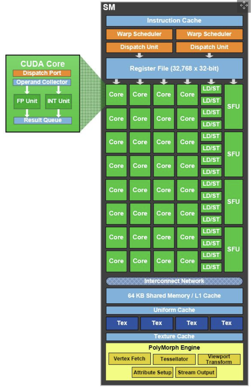
Fig. 118 Streaming Multiprocessor SM figure from book [81].¶ |
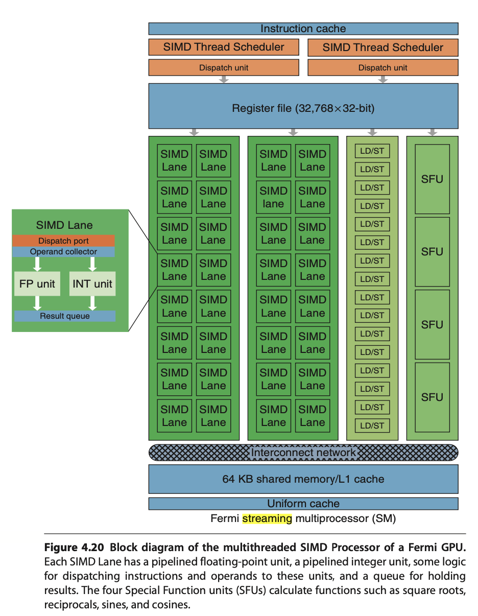
|
Streaming Multiprocessor SM has two 16-way SIMD units and four special function units. Fermi has 32 SIMD Lanes and Cuda cores. SM has L1 and Read Only Cache (Uniform Cache) GTX480 has 48 SMs.
In Fermi, ALUs run at twice the clock rate of rest of chip. So each decoded instruction runs on 32 pieces of data on the 16 ALUs over two ALU clocks [79]. However after Fermi, the ALUs run at the same clock rate of rest of chip.
As Fig. 118 in Fermi and Volta, it can dual-issue “float + integer” or “integer + load/store” but cannot dual-issue “float + float” or “int + int”.
Uniform cache: used for storing constant variables in OpenGL (see uniform of Pipeline Qualifiers) and in OpenCL/CUDA.
Configurable maximum resident warps and allocated registers per thread as follows:
Example: Fermi SM (SM 2.x)
Hawdware limit:
Total registers per SM = 32,768 × 32-bit
Max Warps per SM = 48
Max threads per SM = 1536
Max registers/thread = 63
Configuration: If each thread uses R registers:
Max resident threads = floor(32768 / R)
Max resident Warps = floor(Max resident threads / 32)
E.g. R=32: Max resident threads = 32768/32 = 1024, Max resident Warps = 1024/32 = 32.
After Fermi, the hardware limit for Maxwell, Pascal, Volta and Ampere are:
Hawdware limit:
Each SM includes 32 Cuda cores and Lanes → 32 active threads.
Total registers per SM = 64K x 32-bit
Max Warps per SM = 64
Max threads per SM = 2048 (64 Warps x 32 threads)
Max registers/thread = 255
Notes:
Registers per thread: max number of registers compiler can allocate to a thread.
The “registers per thread” limit (255) is a hardware/compiler limit, but the actual number used depends on the kernel. If a kernel uses too many registers per thread, occupancy drops (fewer threads can be resident).
The “max threads per SM = 2048” is a theoretical upper limit; actual resident threads will also depend on shared memory usage, number of thread-blocks per SM, and register usage.
Note
A SIMD thread executed by a Multithreaded SIMD processor, also known as an SM, processes 32 elements.
As configuation above, the 32,768 registers per SM can be configured to each thread alllocated 32 registers, Max resident Warps = 32.
Fermi has a mode bit that offers the choice of using 64 KB of SRAM as a 16 KB L1 cache with 48 KB of Local Memory or as a 48 KB L1 cache with 16 KB of Local Memory [93].
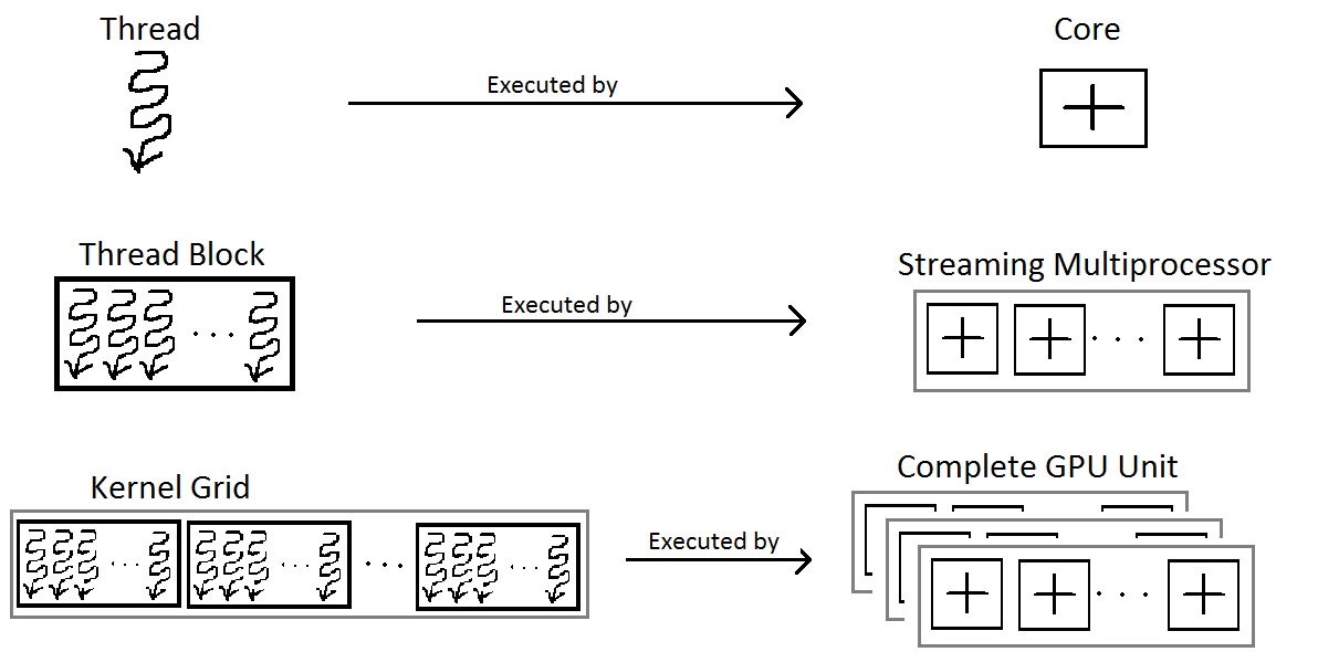
|

|
SM Scheduling
A GPU is built around an array of Streaming Multiprocessors (SMs). A multithreaded program is partitioned into blocks of threads that execute independently from each other, so that a GPU with more multiprocessors will automatically execute the program in less time than a GPU with fewer multiprocessors [76].
Nvidia’s GPUs:
Fermi (2010), Kepler (2012), Maxwell (2014), Pascal (2016), Volta (2017), Turing (2018), Ampere (2020), Ada Lovelace (2022), and Hopper (2022, for data centers).
Two levels of scheduling:
Level 1: Thread Block Scheduler
For Fermi/Kepler/Maxwell/Pascal (pre-Volta): Warp-synchronous SIMT (lock-step in Warp):
A Warp includes 32 threads in Fermi GPU. Each Streaming Multiprocessor SM includes 32 Lanes in Fermi GPU, as shown in Fig. 120, the Thread Block includes a Warp (32 threads). According Fig. 121, more than one block can be assigned and run on a same SM.
When an SM executes a Thread Block, all the threads within the block are are executed at the same time. If any thread in a Warp is not ready due to operand data dependencies, the scheduler switches context between Warps. During a context switch, all the data of the current Warp remains in the register file so it can resume quickly once its operands are ready [100].
Once a Thread Block is launched on a multiprocessor (SM), all of its Warps are resident until their execution finishes. Thus a new block is not launched on an SM until there is sufficient number of free registers for all Warps of the new block, and until there is enough free shared memory for the new block [100].
Level 2: Warp Scheduler
Manages CUDA threads (resident threads) within the same Warp.
A resident thread is a thread whose execution context has been allocated on an SM (registers, Warp slot, shared memory). Once resident, the thread is always in exactly one of the following execution states.
Resident Thread
├── Ready
│     Thread is eligible to execute; no pending dependencies.
│
├── Running
│     Warp containing the thread is currently issued by the scheduler.
│
│     ├── Active (mask = 1)
│     │     Thread participates in the current instruction.
│     │
│     └── Inactive (mask = 0)
│           Thread is masked off due to branch divergence and
│           will re-activate at a reconvergence point.
│
├── Stalled
│     Warp cannot issue due to memory latency, synchronization,
│     or scoreboard dependency.
│
└── Exited
      Thread has completed execution but its Warp has not yet been
      released from the SM.
Threads retain their registers and per-thread local memory during the stalled state. Therefore, the context switch incurs almost no overhead compared to CPU threads.
No pipeline flush: illustrate below.
No register save/restore
No stack frame swapping
No OS involvement
Takes roughly 1 cycle
No pipeline flush because:
For Fermi/Kepler/Maxwell/Pascal (pre-Volta): Warp-synchronous SIMT (lock-step in Warp):
No data is saved/restored when switching to another Warp
Switching Warps = selecting a different Warp in the Warp scheduler
No pipeline flush
On an NVIDIA GPU, no pipeline flush occurs when a Warp stalls because the Warp’s next instruction is never issued until its operands are ready as illustrated in Warp scheduling in Level 1. The stalled Warp simply stops issuing instructions, and its pipeline slot is taken by another ready Warp. When the stall condition clears, the Warp re-enters the pipeline by issuing the stalled instruction anew. No state is saved or restored.
For Volta, Turing, Ampere, Hopper: Independent Thread Scheduling:
No pipeline flush
Stalled threads simply do not issue instructions.
Other threads in the same warp continue issuing independently.
No pipeline flush needed and No data is saved/restored because instructions are tracked per thread, not per warp.
SIMT and SPMD Pipelines
This section illustrates the difference between SIMT and SPMD pipelines using the same pipeline stages: Fetch (F), Decode (D), Execute (E), Memory (M), and Writeback (W).
A GPU contains many SMs. The execution model between SMs is MIMD (Multiple Instructions, Multiple Data) when running different programs, or SPMD (Single Program, Multiple Data). However, within a single SM, the execution model is SIMD/SIMT.”
Low-end GPUs implement SIMD in their pipelines, where all instructions are executed in lockstep. High-end GPUs, however, approximate SPMD in their pipelines, meaning that instructions are interleaved within the pipeline, as shown below.
SPMD Programming Model vs SIMD/SIMT Execution
In the SISD of CPU, a thread is a single pipeline execution unit which can be issued at any specific address.
In a multi-core CPU running SPMD, each core can schedule and execute instructions at any program counter (PC). For example, core-1 may execute I(1–10), while core-2 executes I(31–35). For GPU, however, within an SM, it is not possible to schedule thread-1 to execute I(1–10) while thread-2 executes I(31–35).
As result, there is no mainstream GPU that is truly hardware-SPMD (where each thread has its own independent pipeline). All modern GPUs (NVIDIA, AMD, Intel) implement SPMD as a programming model, but under the hood they execute in SIMD lock-step groups (Warps or Wavefronts). GPUs expose an SPMD programming model (each thread runs the same kernel on different data). However, the hardware actually executes instructions in SIMD/SIMT lock-step groups.
An example to illustrate the difference between Pascal SIMT, Volta SIMT and SPMD.
Divergent Kernel Example:
-------------------------
if (tid % 2 == 0) {         // even threads: long loop
  for (...) { loop_body } // many iterations
} else {                    // odd threads: short path
  C[tid] = A[tid] + B[tid];
}

Legend: F=Fetch, D=Decode, E=Execute, M=Memory, W=Writeback
        S=Stall/masked-off, "..." = loop continues


===================================================================
Pascal (lock-step SIMT with SIMT stack)
-------------------------------------------------------------------
Cycle →   0   1   2   3   4   5   6   7   8   9  10  11  12 ...
T0 even:  F   D   E   M   W   F   D   E   M   W   F   D  ...
T1 odd :  S   S   S   S   S   S   S   S   S   S   S   S  ...
          (Odd threads wait until even path completes, then:)
          ... F D E M W → done


===================================================================
Volta (SIMT with independent thread scheduling)
-------------------------------------------------------------------
Cycle →   0   1   2   3   4   5   6   7   8   9  10  11 ...
T0 even:  F   D   E   M   W   F   D   E   M   W   F   D  ...
T1 odd :      F   D   E   M   W   done
          (Odd thread issues its short path early,
           interleaved with even loop instructions)


===================================================================
True SPMD (CPU-like, fully independent threads)
-------------------------------------------------------------------
Cycle →   0   1   2   3   4   5   6   7   8   9 ...
T0 even:  F   D   E   M   W   F   D   E   M   W  ...
T1 odd :  F   D   E   M   W   done
          (Threads fetch/execute independently —
           odd thread finishes immediately)
Note
SPMD and MIMD
When run a single program across all cores, SPMD and MIMD pipelines look the same.
The subection Mapping data in GPU includes more details in Lanes masked.
Scoreboard purpose:
GPU scoreboard = in-order issue, out-of-order completion
CPU reorder buffer (ROB) = out-of-order issue + completion, but retire in-order - CPUs use a ROB to support out-of-order issue and retirement.
Comparsion of Volta and Pascal
In a lock-step GPU without divergence support, the scoreboard entries include only {Warp-ID, PC (Instruction Address), …}. With divergence support (as in real-world GPUs), the scoreboard entries expand to {Warp-ID, PC, mask, …}.
Volta (Cuda thread/SIMD Lane with PC, Program Couner and Call Stack)
GPU scoreboard = in-order issue, out-of-order completion
SIMT GPU before Volta = scoreboard contains: { Warp ID + PC + Active Mask }
Volta = scoreboard contains: { Warp ID + PC per thread (+ readiness per thread) }
Example for mutex [103]
//
__device__ void insert_after(Node *a, Node *b)
{
  Node *c;
  lock(a); lock(a->next);
  ...
  unlock(c); unlock(a);
}
Assume that the mutex is contended across SMs but not within the same SM. On average, each thread spends 10 cycles executing the insert_after operation without resource contention, and 20 cycles when accounting for contention. Therefore, the average total execution time for 32 threads in an SM is:
Volta: 20 cycles
Pascal: 640 cycles (20 cycles × 32 threads, due to lack of independent progress inside a Warp)
Processor Units and Memory Hierarchy in NVIDIA GPU [82]
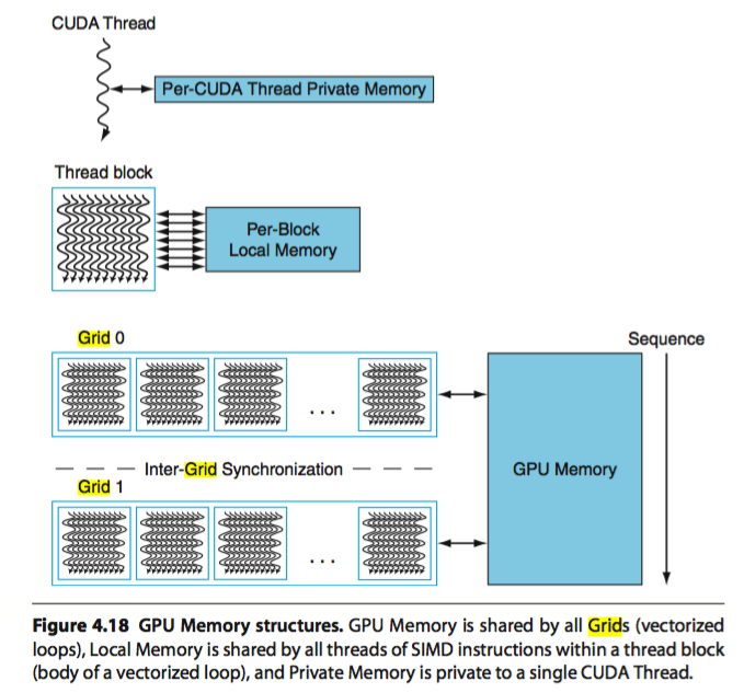
![digraph GPU_Memory_Hierarchy {
rankdir=TB;
node [shape=box, style=rounded, fontname="Helvetica"];
// Processing hierarchy
GigaThread [label="GigaThread Engine\n(Chip-wide Scheduler)"];
GPC [label="GPC\n(Graphics Processing Cluster)"];
TPC [label="TPC\n(Texture Processing Cluster)"];
SM [label="SM\n(Streaming Multiprocessor)"];
Core [label="CUDA Cores"];
// Memory hierarchy
Global [label="Global Memory (HBM/GDDR)\nGPU-wide, slowest"];
L2 [label="L2 Cache\nGPU-wide"];
L1 [label="L1 Cache\nPer-SM, unified with Shared"];
Uniform [label="Uniform / Constant Cache\nPer-SM, Read-only,\nFor Uniform Parameters"];
Shared [label="Shared Memory\nPer-SM, Block-visible"];
Local [label="Local Memory\nPer-thread, in DRAM"];
Reg [label="Registers\nPer-thread, fastest"];
// Hierarchy connections
GigaThread -> GPC -> TPC -> SM -> Core;
// Memory hierarchy connections
Global -> L2;
L2 -> L1;
L2 -> Uniform;
L1 -> Core;
Uniform -> Core;
Shared -> SM;
Reg -> Core;
Local -> Core;
// Styling groups
subgraph cluster_gpu {
label="GPU Processing Units";
style=dashed;
GigaThread; GPC; TPC; SM; Core;
}
subgraph cluster_mem {
label="Memory Hierarchy";
style=dashed;
Global; L2; L1; Uniform, Shared; Local; Reg;
}
}](_images/graphviz-5ce62e2d24d290889b7c0e7f71d9f21cfb84e1f3.png)
Fig. 123 Processor Units and Memory Hierarchy in NVIDIA GPU Local Memory is shared by all threads and Cached in L1 and L2. In addition, the Shared Memory is provided to use per-SM, not cacheable.
Illustrate L1, L2 and Global Memory used by SM and whole chip of GPU as Fig. 124.

Fig. 124 L1 Cache: Per-SM, Coherent across all 16 Lanes in the same SM. L2 Cache: Coherent across all SMs and GPCs. Global Memory (DRAM: HBM/GDDR). Both HBM and GDDR are DRAM. GDDR (Graphics DDR) – optimized for GPUs (GDDR5, GDDR6, GDDR6X). HBM (High Bandwidth Memory) – 3D-stacked DRAM connected via TSVs (Through-Silicon Vias) for extremely high bandwidth and wide buses [76].
The Fig. 123 illustrates the memory hierarchy in NVIDIA GPU. The Cache flow for 3D Model Information, Animation Parameters, and GLSL Variables is as follows:
- 3D Model Information:
VBO/IBO → Global → L2 → L1 → Registers
Material constants → Uniform Cache → Registers
- Animation Parameters:
Bone matrices → Uniform Cache → Registers
Morph targets → Global → L2 → L1 → Registers
Shared bone data (compute) → Shared Memory
- GLSL Variables:
uniform → Uniform Cache
in (vertex attributes) → Global → L2 → L1
out (varyings) → Registers → Interpolators
buffer (SSBO) → Global → L2 → L1
shared → Shared Memory
local arrays → Registers or Local Memory
More details of the NVIDIA GPU memory hierarchy are described as follows:
Registers
Per-thread, fastest memory, located in CUDA cores, as illustrated also in Fig. 118.
Configurable maximum resident warps and allocated registers per thread following Fig. 118.
Latency: ~1 cycle.
Uniform / Constant cache
Stored constant variables in OpenGL and OpenCL/CUDA, as illustrated in Fig. 118.
Local Memory
Per-thread, stored in global DRAM.
Cached in L1 and L2.
Latency: high, depends on cache hit/miss.
Shared Memory
Per-SM, shared across threads in a Thread Block as shown in Fig. 118.
On-chip, programmer-controlled.
Latency: ~20 cycles.
L1 Cache
Per-SM, unified with shared memory.
Hardware-managed.
Latency: ~20 cycles.
L2 Cache
Shared across the entire GPU chip.
Coherent across all SMs and GPCs as shown in Fig. 124.
Global Memory (DRAM: HBM/GDDR)
Visible to all SMs across all GPCs.
Highest latency (~400–800 cycles).
GPU Hierarchy Context
GigaThread Engine (chip-wide scheduler)
Contains multiple GPCs.
Fermi (2010): up to 4 GPCs per chip.
Pascal GP100 (Tesla P100): 6 GPCs.
Volta GV100 (Tesla V100): 6 GPCs.
Distributes Thread Blocks to all GPCs.
GPC (Graphics Processing Cluster)
Contains multiple TPCs.
TPC (Texture Processing Cluster)
Groups 1–2 SMs.
SM (Streaming Multiprocessor)
Contains CUDA cores, registers, shared memory, L1 cache.
CUDA Cores
Execute threads with registers and access the memory hierarchy.
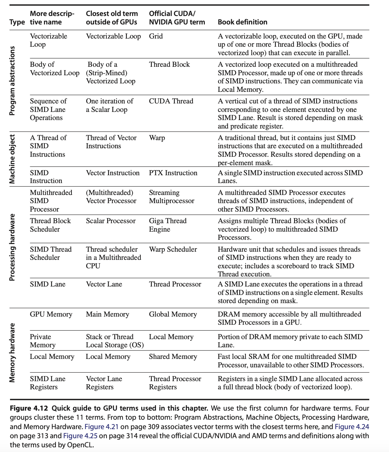
![digraph WarpSchedulerPipeline {
rankdir=TB;
node [shape=box, style=filled, fillcolor=lightgray];
WarpScheduler -> InstructionIssue;
InstructionIssue -> Lane0;
InstructionIssue -> Lane1;
InstructionIssue -> Lane2;
InstructionIssue -> Lane3;
InstructionIssue -> Lane4;
InstructionIssue -> Lane5;
InstructionIssue -> Placeholder;
InstructionIssue -> Lane30;
InstructionIssue -> Lane31;
Lane0 [label="Lane 0\n(Chime A / Chime B)", fillcolor=lightyellow];
Lane1 [label="Lane 1\n(Chime A / Chime B)", fillcolor=lightyellow];
Lane2 [label="Lane 2\n(Chime A / Chime B)", fillcolor=lightyellow];
Lane3 [label="Lane 3\n(Chime A / Chime B)", fillcolor=lightyellow];
Lane4 [label="Lane 4\n(Chime A / Chime B)", fillcolor=lightyellow];
Lane5 [label="Lane 5\n(Chime A / Chime B)", fillcolor=lightyellow];
Placeholder [label="………………", shape=plaintext, fillcolor=white];
Lane30 [label="Lane 30\n(Chime A / Chime B)", fillcolor=lightyellow];
Lane31 [label="Lane 31\n(Chime A / Chime B)", fillcolor=lightyellow];
}](_images/graphviz-cc2f17258f647668997d9703e4ad9c88e4df68ce.png)
Fig. 126 In dual-issue mode, Chime A carries floating-point data while Chime B carries integer data—both issued by the same CUDA thread. In contrast, under time-sliced execution, Chime A and Chime B carry either floating-point or integer data independently, and are assigned to separate CUDA threads.
A Warp of 32 threads is mapped across 16 Lanes. If each Lane has 2 Chimes, it may support dual-issue or time-sliced execution as Fig. 126.
In the following matrix multiplication code, the 8096 elements of matrix A = B × C are mapped to Thread Blocks, SIMD Threads, Lanes, and Chimes as illustrated in the Fig. 127. In this example, it run on time-sliced execution.
// Invoke MATMUL with 256 threads per Thread Block
__host__
int nblocks = (n + 255) / 512;
matmul<<<nblocks, 255>>>(n, A, B, C);
// MATMUL in CUDA
__device__
void matmul(int n, double A, double *B, double *C) {
  int i = blockIdx.x*blockDim.x + threadIdx.x;
  if (i < n) A[i] = B[i] + C[i];
}
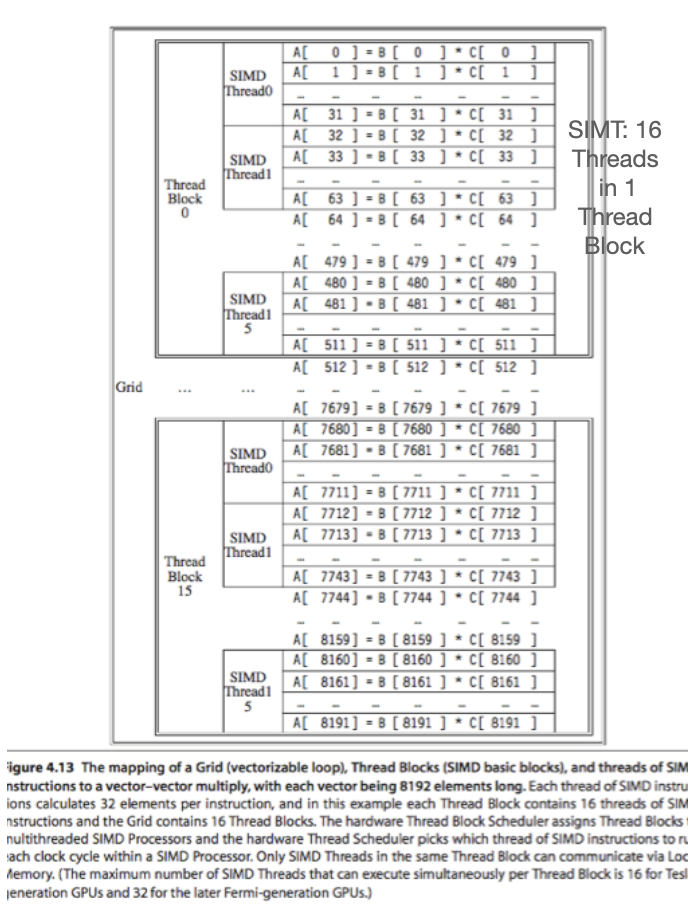
Fig. 127 Mapping 8192 elements of matrix multiplication for Nvidia’s GPU (figure from [75]). SIMT: 16 SIMD threads in one Thread Block.
Explain the mapping and execution in Fig. 127 for MATMUL CUDA Example using the terminology from Fig. 125 and the previous sections of this book, presented in the table below.
Terms |
Structure |
Description |
|---|---|---|
Grid, Giga Thread Engine |
Each loop (Grid) consists of multiple Thread Blocks. |
Grid is Vectorizable Loop as Fig. 125. The hardware scheduler Guda Thread Engine schedules the Thread Blocks to SMs. |
Thread Block |
In this example, each Grid has 16 Giga Thread [95]. |
Each Thread Block is assigned 512 elements of the vectors to work on. As Fig. 127, it assigns 16 Thread Block to 16 SMs. Giga Thread is the name of the scheduler that distributes Thread Blocks to Multiprocessors, each of which has its own SIMD Thread Scheduler [95]. More than one Block can be mapped to a same SM as the explanation in “Level 1: Thread Block Scheduler” for Fig. 121. |
Streaming Multiprocessor, SM, GPU Core (Warp) [101] |
Each SIMD Processor has 16 SIMD Threads. |
Each SIMD processor includes local memory, as in Fig. 122. Local memory is shared among SIMD Lanes within a SIMD processor but not across different SIMD processors. A Warp has its own PC and may correspond to a whole function or part of a function. Compiler and runtime may assign functions to the same or different Warps [102]. |
Cuda core |
Fermi has 32 Cuda cores in a SM as Fig. 119. |
A CUDA core is the scalar execution unit inside an SM. It is capable of executing one integer or floating-point instruction from one Lane of a Warp. The CUDA core is analogous to an ALU pipeline stage in a CPU. |
Cuda Thread |
Each SM can configure to have different number of resident threads. |
Fermi can configure Max resident threads = 32768/32 = 1024 for 32 registers/per thread in a SM as memtioned eariler. A CUDA thread is the basic unit of execution defined in CUDA’s programming model. Each thread executes the kernel code independently with its own registers, program counter (PC), and per-thread local memory. Each Thread has its TLR (Thread Level Registers) allocated from Register file (32768 x 32-bit) by SIMD Processor (SM) as Fig. 118. |
SIMD Lane |
Each SIMD Thread has 32 Lanes. |
A vertical cut of a thread of SIMD instructions corresponding to one element executed by one SIMD Lane. It is a vector instruction with processing 32-elements. A Warp of 32 threads is mapped across 32 Lanes. Lane = per-thread execution slot inside a Warp. If each Lane has 2 Chimes, it may support dual-issue or time-sliced execution as Fig. 126. |
Chime |
Each Lane has 2 Chimes. |
A Chime represents one “attempt” or opportunity for issuing instructions from Warps. In Fermi (SM2.x): Each SM has 2 Warp schedulers. Each Warp scheduler has 2 dispatch units (dual-issue, but with constraints, it can issue “float + load/store” for “fadd and load C[i]” in this example). |
References
Memory Subsystem
Address Coalescing and Gather-scatter
Brief description is shown in Fig. 128.
![digraph GPU_Memory {
rankdir=LR;
node [shape=box, style=rounded, fontsize=12];
subgraph cluster_gather {
label="Gather-Scatter (Sparse Matrix Access): \nIndirect index of LD/ST";
color=green;
Idx [label="Index Array A[]:\nA[0]=200\nA[1]=400\nA[2]=1200\nA[3]=320", shape=note, style=filled, fillcolor=lightyellow];
G1 [label="Thread 1\nMem[A[0]]"];
G2 [label="Thread 2\nMem[A[1]]"];
G3 [label="Thread 3\nMem[A[2]]"];
G4 [label="Thread 4\nMem[A[3]]"];
Idx -> G1;
Idx -> G2;
Idx -> G3;
Idx -> G4;
}
subgraph cluster_coalescing {
label="Address Coalescing: \nMerge memory transcations into a contiguous memory access";
color=blue;
T1 [label="Thread 1\nAddr 100"];
T2 [label="Thread 2\nAddr 104"];
T3 [label="Thread 3\nAddr 108"];
T4 [label="Thread 4\nAddr 112"];
MT [label="Merged Transaction", shape=ellipse, style=filled, fillcolor=lightblue];
T1 -> MT;
T2 -> MT;
T3 -> MT;
T4 -> MT;
T5 [label="Addr[100..112]", shape=ellipse, style=filled, fillcolor=lightblue];
MT -> T5;
}
}](_images/graphviz-a9d0800a94d34796e0dcd9d6ad5e1d283861694c.png)
Fig. 128 Coalescing and Gather-scatter
The Load/Store Units (LD/ST) is important because memory latency is huge compared to ALU ops. Some GPUs provide Address Coalescing and gather-scatter to accelerate memory access.
Address Coalescing: Memory coalescing is the process of merging memory requests from threads in a Warp (NVIDIA: 32 threads, AMD: 64 threads) into as few memory transactions as possible.
Cache miss (global memory/DRAM): Coalescing = big performance improvement.
Cache hit (L1/L2): Coalescing = smaller benefit, since cache line fetch already amortizes cost.
Note that unlike vector architectures, GPUs don’t have separate instructions for sequential data transfers, strided data transfers, and gather-scatter data transfers. All data transfers are gather-scatter! To regain the efficiency of sequential (unit-stride) data transfers, GPUs include special Address Coalescing hardware to recognize when the SIMD Lanes within a thread of SIMD instructions are collectively issuing sequential addresses. That runtime hardware then notifies the Memory Interface Unit to request a block transfer of 32 sequential words. To get this important performance improvement, the GPU programmer must ensure that adjacent CUDA Threads access nearby addresses at the same time that can be coalesced into one or a few memory or cache blocks, which our example does [99].
Gather-scatter data transfer: HW support sparse vector access is called gather-scatter. The VMIPS instructions are LVI (load vector indexed or gather) and SVI (store vector indexed or scatter) [98].
1. Address Coalescing in GPU Memory Transactions
Definition: Memory coalescing is the process of merging memory requests from threads in a Warp (NVIDIA: 32 threads, AMD: 64 threads) into as few memory transactions as possible.
How It Works:
If threads access contiguous and aligned addresses, the hardware combines them into a single memory transaction.
If threads access strided or random addresses, the GPU must issue multiple transactions, wasting bandwidth.
Examples:
Coalesced (efficient):
// Each thread accesses consecutive elements
value = A[threadId];
→ One transaction for 32 threads.
Non-coalesced (inefficient):
// Each thread accesses strided elements
value = A[threadId * 100];
→ Many transactions required due to striding.
2. Gather–Scatter in Sparse Matrix Access
Definition: Gather–scatter refers to memory operations where each GPU thread in a Warp loads from or stores to irregular memory addresses. This is common in sparse matrix operations, where non-zero elements are stored in compressed formats.
Sparse Matrix Example (CSR format):
CSR (Compressed Sparse Row) stores three arrays:
values[]: non-zero entries of the matrixcolIndex[]: column indices for each non-zerorowPtr[]: index intovalues[]for each row
Sparse matrix-vector multiplication (SpMV):
for row in matrix:
    for idx = rowPtr[row] to rowPtr[row+1]:
        col = colIndex[idx];      // gather index
        val = values[idx];        // gather nonzero
        y[row] += val * x[col];   // scatter result
Characteristics:
Gather: Each thread loads from potentially scattered locations (
values[idx]orx[col]).Scatter: Results may be written back to irregular output locations (
y[row]).Challenge: These accesses often break memory coalescing, leading to multiple memory transactions. An example is shown as follows:
Summary:
Gather–scatter is fundamental for sparse matrix access but typically results in non-coalesced memory patterns.
Address coalescing is critical for high GPU throughput; restructuring data to improve coalescing often provides significant performance gains.
VRAM dGPU
![digraph gpu_memory {
rankdir=LR;
node [shape=box style=rounded fontsize=10];
subgraph cluster_shared {
label = "Shared Memory (Integrated GPU)";
CPU [label="CPU\n(Caches, DMA)"];
GPU [label="iGPU\n(DMA Engine)"];
MC [label="Shared\nMemory Controller"];
DRAM [label="System RAM\n(DDR/LPDDR)"];
CPU -> MC -> DRAM;
GPU -> MC;
GPU -> DRAM [style=dashed, label="DMA"];
}
subgraph cluster_dedicated {
label = "Dedicated Memory (Discrete GPU)";
CPU2 [label="CPU\n(Caches)"];
SYS_RAM [label="System RAM"];
GPU2 [label="dGPU\n(Caches, DMA)"];
VRAM [label="VRAM\n(GDDR/HBM)"];
CPU2 -> SYS_RAM;
GPU2 -> VRAM;
}
edge [style=invis];
DRAM -> CPU2;
}](_images/graphviz-328629f7399688d6d95bdb0681815ab51799ec25.png)
Fig. 129 iGPU versus dGPU
Reason:
1. Since CPU and GPU have different requirements, a shared memory design cannot match the performance of dedicated GPU memory.
2. In systems with shared memory (like integrated GPUs), both the CPU and GPU access the same physical memory (DRAM). This leads to several forms of contention:
Cache Coherency Overhead
DMA Contention
Bus & Memory Controller Bottleneck
Advantages:
A discrete GPU has its own dedicated memory (VRAM) while an integrated GPU (iGPU) shares memory with the CPU as shown in Fig. 129.
Dedicated GPU memory (VRAM) outperforms shared CPU-GPU memory due to higher bandwidth, lower latency, parallel access optimization, and no contention with CPU resources.
Feature |
Shared Memory (CPU + iGPU) |
Dedicated GPU Memory (dGPU) |
|---|---|---|
Bandwidth |
Lower (DDR/LPDDR) |
Higher (GDDR/HBM) |
Latency |
Higher |
Lower |
Parallel Access |
Limited |
Optimized for many threads |
Cache Coherency |
Required (with CPU) |
Not required |
DMA Bandwidth |
Shared with CPU |
GPU has exclusive DMA access |
Memory Contention |
Yes |
No |
Performance |
Lower: Bandwidth bottlenecks, CPU-GPU interference and Cache/DMA conflicts |
Higher: Wide memory bandwidth, Parallel thread access and Low latency memory access |
Dedicated memory allows the GPU to run high-throughput workloads without interference from the CPU. It provides (1). wide bandwidth, (2). optimized parallel access, and (3). low-latency paths, avoiding cache and DMA conflicts for superior performance.**
(1). Wide bandwidth: Dedicated GPU memory (VRAM) is often based on GDDR6, GDDR6X, or HBM2/3, which are much faster than standard system RAM (DDR4/DDR5).
Typical bandwidths:
GDDR6: ~448–768 GB/s
HBM2: up to 1 TB/s+
DDR5 (shared memory): ~50–80 GB/s
Impact: Faster access to textures, vertex buffers, and framebuffers—critical for rendering and compute tasks.
(2). Optimized parallel access:
VRAM is optimized for the massively parallel architecture of GPUs.
It allows thousands of threads to access memory simultaneously without stalling.
Shared system memory is optimized for CPU access patterns, not thousands of GPU threads.
(3). Low-latency paths:
Dedicated memory is physically closer to the GPU die.
No need to traverse the PCIe bus like discrete GPUs accessing system RAM.
In shared memory systems (like integrated GPUs), memory access may have to go through a memory controller shared with the CPU, adding delay.
RegLess-style architectures [47]
Note
RegLess remains a research concept, not (as far as public evidence shows) a commercial design in shipping GPUs.
Difference: Add Staging Buffer between Register Files and Execution Unit.
This section outlines the transition from traditional GPU operand coherence using a monolithic register file and L1 data cache, to a RegLess-style architecture that employs operand staging and register file-local coherence.
✅ Operand Delivery in Traditional GPU: Fig. 130:
![digraph TraditionalOperandDelivery {
rankdir=LR;
node [shape=box, style=filled, fontname="Helvetica", fontsize=10];
subgraph cluster_memory {
label="Memory Hierarchy";
style=filled;
color=lightgray;
GMEM [label="Global Memory"];
L1 [label="L1 Cache", fillcolor=lightyellow];
}
subgraph cluster_registers {
label="Register File";
style=filled;
color=lightblue;
RF [label="Register File"];
}
subgraph cluster_execution {
label="Execution Pipeline";
style=filled;
color=lightgreen;
EU [label="Execution Unit"];
}
GMEM -> L1 [label="Coherence (Hardware-managed)", color=blue];
L1 -> RF [label="LD/ST (Compiler-controlled)", style=dashed];
RF -> EU [label="Operands"];
L1 -> EU [label="Cached Data (optional)", style=dashed];
}](_images/graphviz-0d852fae840859fab4ab7f9eaf50d587dff69295.png)
Fig. 130 Operand Delivery in Traditional GPU (Traditional Model: Register File + L1 Cache)
- Architecture:
Large monolithic register file per SM (e.g., 256KB, Maxwell, Pascal, Volta and Ampere have 64K x 32-bit register file per SM, see Configurable maximum resident warps and allocated registers per thread)
Coherent with L1 data cache via write-through or write-back policies
- Challenges:
High energy cost due to cache coherence traffic
Complex invalidation and synchronization logic
Register pressure limits Warp occupancy (limit the number of ative Warps)
Redundant operand tracking across register file and cache
Example:
v1 = normalize(N)
v2 = normalize(L)
v3 = dot(v1, v2)
v4 = max(v3, 0.0)
v5 = mul(v4, color)

# All operands reside in register file and may be cached in L1
✅ Operand Delivery in RegLess GPU (with L1 Cache in LD Path): Fig. 131:
![digraph RegLessOperandDeliveryWithL1 {
rankdir=LR;
node [shape=box, style=filled, fontname="Helvetica", fontsize=10];
subgraph cluster_memory {
label="Memory Hierarchy";
style=filled;
color=lightgray;
GMEM [label="Global Memory"];
L1 [label="L1 Cache", fillcolor=lightyellow];
}
subgraph cluster_registers {
label="Register File";
style=filled;
color=lightblue;
RF [label="Register File"];
}
subgraph cluster_execution {
label="Execution Pipeline";
style=filled;
color=lightgreen;
SB [label="Staging Buffer"];
EU [label="Execution Unit"];
}
GMEM -> L1 [label="Coherence (Hardware-managed)", color=blue];
L1 -> RF [label="Operand Fetch (via LD)", style=dashed];
RF -> SB [label="Staging (Just-in-Time)", style=dashed];
SB -> EU [label="Transient Operands"];
RF -> EU [label="Persistent Operands"];
RF -> RF [label="Internal Coherence", color=green];
}](_images/graphviz-579c89897fc8057adcc00f3a7679c101c035d00f.png)
Fig. 131 Operand Delivery in RegLess GPU (with L1 Cache in LD Path)
Description
Global Memory: Source of all operands and data.
L1 Cache: Participates in memory hierarchy; may serve LD requests.
Register File: Receives operands via LD; stages them into Staging Buffer for Transient Operands.
Staging Buffer: Holds transient operands for immediate execution.
Execution Unit: Consumes operands from Staging Buffer for Transient Operands and Register File for Persistent Operands.
Notes
L1 Cache is not part of staging—it only serves LDs.
Dashed arrows: Compiler-controlled operand movement.
Solid arrows: Operand delivery to execution.
Green self-loop: Internal coherence within Register File.
RegLess Model: Staging-Aware Register File
- Architecture:
Smaller register file (e.g., 64–128KB per SM)
For Transient Operands, no L1 cache coherence required
Operands staged dynamically based on lifetime
- Key Concepts:
Region slicing: compiler divides computation into operand regions
Operand tagging: transient, intermediate, persistent
Metadata compression: region-level hints, not per-instruction lifetimes
- Benefits:
~75% reduction in register file size
~11% energy savings
Simplified coherence model
Improved Warp occupancy
Example with Operand Staging:
v1 = normalize(N)         # transient
v2 = normalize(L)         # transient
v3 = dot(v1, v2)          # intermediate
v4 = max(v3, 0.0)         # intermediate
v5 = mul(v4, color)       # persistent

# v1 and v2 staged briefly, v3–v4 may be staged or registered, v5 fully
# registered
Compiler-Hardware Interface
- Compiler Responsibilities:
Emit structured IR with operand usage hints
Slice computation graph into regions
Avoid explicit staging register allocation
- Hardware Responsibilities:
Interpret operand lifetime metadata
Dynamically stage operands or allocate registers
For Transient Operands, eliminate L1 cache coherence logic
- Metadata Compression Techniques:
Region-level tagging
Operand class encoding
Profile-guided optimization
Off-chip metadata tables (e.g., DEER)
Conclusion
The move to RegLess-style coherence simplifies GPU operand management, reduces energy, and enables more efficient shader execution. Compiler-guided operand staging and region slicing allow hardware to dynamically optimize operand placement without burdening the instruction stream with excessive metadata.
Specialized Units
As shown in section GPU Hardware Units, the stages of the OpenGL rendering pipeline and the GPU hardware units that accelerate them as shown in Fig. 132:
Fig. 132 The stages of OpenGL pipeline and GPU’s acceleration components
We now explain how these GPU hardware acceleration units—Geometry Units, Rasterization Units, Texture Mapping Units (TMUs), and Render Output Units (ROPs) —- work together with SMs to provide GPU-ISA instructions that accelerate the graphics pipeline illustrated in Fig. 133 of section 3D Rendering.
Figure illustrated in section 3D Rendering
Geometry Units
Function:
Raw Vertices & Primitives → Transformed Vertices & Primitives
Suppose the GLSL geometry shader looks like this:
An example of GLSL geometry shader
#version 450
layout(triangles) in;
layout(line_strip, max_vertices = 2) out;

void main() {
  gl_Position = gl_in[0].gl_Position;
  EmitVertex();

  gl_Position = gl_in[1].gl_Position;
  EmitVertex();

  EndPrimitive();
}
The corresponding PTX instructions and pipeline flow as Fig. 134.
![digraph SM_Geometry_Assembly {
rankdir=LR;
bgcolor="white";
node [shape=box, style="rounded,filled", fontname="Arial", fontsize=11];
/* Graph-level title (left-aligned, bold) */
label=<
<TABLE BORDER="0" CELLBORDER="0" CELLSPACING="0" ALIGN="LEFT">
<TR><TD><FONT POINT-SIZE="14" COLOR="#003366"><B>SM → Geometry Unit: PTX-like Assembly Flow</B></FONT></TD></TR>
<TR><TD><FONT POINT-SIZE="10" COLOR="#003366">Example sequence showing loads/moves and {@code call emit}/{@code call cut} dispatching primitives</FONT></TD></TR>
</TABLE>
>;
labelloc=top;
/* SM thread node */
SMThread [fillcolor="#FFF2CC" label=<
<TABLE BORDER="0" CELLBORDER="0" CELLSPACING="0" ALIGN="LEFT">
<TR><TD><B>Thread running in SM</B></TD></TR>
<TR><TD>• Executes geometry shader program</TD></TR>
<TR><TD>• Issues compiled PTX-style microcode</TD></TR>
</TABLE>
>];
/* Instruction Fetch / Decoder */
InstFetch [fillcolor="#E6F2FF" label=<
<TABLE BORDER="0" CELLBORDER="0" CELLSPACING="0" ALIGN="LEFT">
<TR><TD><B>Instruction Fetch & Decode</B></TD></TR>
<TR><TD>• Fetches micro-instructions from shader code</TD></TR>
<TR><TD>• Decodes into ALU / LD / CALL operations</TD></TR>
</TABLE>
>];
/* Assembly sequence node showing PTX-like lines */
AsmSeq [fillcolor="#FFFFFF" penwidth="1" label=<
<TABLE BORDER="0" CELLBORDER="0" CELLSPACING="0" ALIGN="LEFT">
<TR><TD><B>Compiled (PTX-like) Instruction Sequence</B></TD></TR>
<TR><TD><FONT FACE="monospace">ld.global.v4.f32 {r0, r1, r2, r3}, [in_attr0];</FONT></TD></TR>
<TR><TD><FONT FACE="monospace">mov.f32 o0, r0;</FONT></TD></TR>
<TR><TD><FONT FACE="monospace">mov.f32 o1, r1;</FONT></TD></TR>
<TR><TD><FONT FACE="monospace">mov.f32 o2, r2;</FONT></TD></TR>
<TR><TD><FONT FACE="monospace">mov.f32 o3, r3;</FONT></TD></TR>
<TR><TD><FONT FACE="monospace"><B>call emit;</B></FONT></TD></TR>
<TR><TD><FONT FACE="monospace">ld.global.v4.f32 {r4, r5, r6, r7}, [in_attr1];</FONT></TD></TR>
<TR><TD><FONT FACE="monospace">mov.f32 o0, r4;</FONT></TD></TR>
<TR><TD><FONT FACE="monospace">mov.f32 o1, r5;</FONT></TD></TR>
<TR><TD><FONT FACE="monospace">mov.f32 o2, r6;</FONT></TD></TR>
<TR><TD><FONT FACE="monospace">mov.f32 o3, r7;</FONT></TD></TR>
<TR><TD><FONT FACE="monospace"><B>call emit;</B></FONT></TD></TR>
<TR><TD><FONT FACE="monospace"><B>call cut;</B></FONT></TD></TR>
</TABLE>
>];
/* Output registers / buffers that hold emitted vertex data */
OutRegs [shape=note, fillcolor="#FFFFE0", label=<
<TABLE BORDER="0" CELLBORDER="0" CELLSPACING="0" ALIGN="LEFT">
<TR><TD><B>Output Registers / Emit Buffer</B></TD></TR>
<TR><TD>• o0..oN hold per-vertex outputs (position, attrs)</TD></TR>
<TR><TD>• Emit buffer queues vertices for Geometry Unit</TD></TR>
</TABLE>
>];
/* Geometry Unit with internal stages (simplified) */
GeoUnit [fillcolor="#D9E8FF" label=<
<TABLE BORDER="0" CELLBORDER="0" CELLSPACING="0" ALIGN="LEFT">
<TR><TD><B>Geometry Unit (hardware)</B></TD></TR>
<TR><TD>• Accepts emitted vertices from SM output regs</TD></TR>
<TR><TD>• Primitive Assembly / Tessellation / GS handling</TD></TR>
<TR><TD>• Culling, Clipping, Viewport transform</TD></TR>
<TR><TD>• Primitive Setup → send to Rasterizer</TD></TR>
</TABLE>
>];
Rasterizer [fillcolor="#F2F8FF" label=<
<TABLE BORDER="0" CELLBORDER="0" CELLSPACING="0" ALIGN="LEFT">
<TR><TD><B>Rasterizer</B></TD></TR>
<TR><TD>• Consumes prepared primitives</TD></TR>
<TR><TD>• Produces fragments for fragment shading</TD></TR>
</TABLE>
>];
/* Dataflow edges */
SMThread -> InstFetch [label=" compiled microcode / instruction pointer" fontsize=10];
InstFetch -> AsmSeq [label=" decode -> micro-ops" fontsize=10];
AsmSeq -> OutRegs [label=" write outputs (o0..oN)" fontsize=10];
OutRegs -> GeoUnit [label=" Emit vertex(s) (emit/cut triggers)" fontsize=10];
GeoUnit -> Rasterizer [label=" prepared primitives" fontsize=10];
/* Control arrows (illustrate call emit/cut semantics) */
AsmSeq -> GeoUnit [label=" call emit / call cut (control msgs)", style=dashed, color="#3333CC"];
/* layout hints */
{ rank = same; SMThread; InstFetch; AsmSeq }
{ rank = same; OutRegs; GeoUnit; Rasterizer }
}](_images/graphviz-e30b52aa74f8c9915dfb4192649b626ef3838cb0.png)
Fig. 134 Fetch a sequence of Geometry instructions and pass to Geometry Unit
The Geometry Unit in a GPU is a collection of fixed-function and programmable stages responsible for transforming assembled primitives (points, lines, triangles, patches) into screen-space primitives ready for rasterization. The emit and cut are compiler intrinsics that map to control messages to the Geometry Unit. When we say emit and cut in NVIDIA PTX (or HLSL/GLSL geometry shaders), they’re not ALU instructions that run in the SM like add or mul. Instead, they act like special control instructions that tell the GPU’s fixed-function Geometry Unit what to do with the vertex data currently in the SM’s output registers illustrated in Fig. 135.
![digraph EmitCut_Flow {
rankdir=LR;
fontsize=12;
labelloc="t";
label="GPU Geometry Shader Dataflow — EmitVertex() and EndPrimitive()";
node [shape=box, style=rounded, fontname="Helvetica"];
subgraph cluster_shader {
label="Streaming Multiprocessor (SM)";
color=lightblue;
style=filled;
fillcolor="#D8EFFF";
thread [label="Shader Thread\n(Geometry Shader Instructions)", shape=box];
emit [label="EmitVertex()\n• write varyings\n• commit vertex", shape=box];
cut [label="EndPrimitive()\n• mark primitive boundary", shape=box];
thread -> emit -> cut;
}
subgraph cluster_fifo {
label="On-Chip FIFO / URB / LDS Buffer";
color=gray;
style=filled;
fillcolor="#EEEEEE";
fifo [label="FIFO Buffer\n(Holds emitted vertices\nand primitive markers)", shape=box];
}
subgraph cluster_geom {
label="Geometry Unit / Primitive Assembler";
color=lightgreen;
style=filled;
fillcolor="#E0FFE0";
geom [label="Geometry Unit\n• reads FIFO entries\n• assembles primitives", shape=box];
}
subgraph cluster_rast {
label="Rasterization Pipeline";
color=lightgray;
style=dashed;
rast [label="Rasterizer\n• receives completed\ntriangles/lines", shape=box];
}
// Dataflow edges
emit -> fifo [label="write vertex data"];
cut -> fifo [label="write primitive end marker"];
fifo -> geom [label="fetch vertex packets"];
geom -> rast [label="assembled primitives"];
// Control flow notes
thread -> emit [style=dashed, color=gray, label="shader executes intrinsics"];
geom -> fifo [style=dotted, color=gray, label="read signals / ready flags"];
// Legend
legend [shape=note, label="LEGEND:\nEmitVertex() = vertex data write\nEndPrimitive() = mark primitive end\nSM → FIFO → Geometry Unit → Rasterizer", fontsize=10];
}](_images/graphviz-b2fc4bb5f80934262b52b68b07e831e0834f323a.png)
Fig. 135 Micro-level flow: SM → Geometry Unit via Emit/Cut
Unlike GLSL textures, which are converted into a specific hardware ISA, the Geometry Shader in Fig. 132 maps directly to the Geometry Units instead of the SMs.
Geometry Unit bridges the vertex shading stage and the rasterization stage as shown in Fig. 136.
![digraph Geometry_Unit {
rankdir=TB;
bgcolor="white";
node [shape=box, style="rounded,filled", fontname="Arial", fontsize=14];
/* Graph-level left-aligned title (bold, dark blue) */
label=<
<TABLE BORDER="0" CELLBORDER="0" CELLSPACING="0" ALIGN="LEFT">
<TR>
<TD>
<FONT POINT-SIZE="18" COLOR="#003366"><B>GPU Geometry Unit - internal stages & dataflow</B></FONT>
</TD>
</TR>
<TR>
<TD>
<FONT POINT-SIZE="14" COLOR="#003366">Flow: Vertex output - Primitive Assembly - (Tessellation) - Geometry Shader - Clipping - Viewport Transform - Primitive Setup - Rasterizer</FONT>
</TD>
</TR>
</TABLE>
>;
labelloc=top;
/* External stages (vertex / rasterizer) */
VertexOut [fillcolor="#FFF2CC" label=<
<TABLE BORDER="0" CELLBORDER="0" CELLSPACING="0" ALIGN="LEFT">
<TR><TD><B>Vertex Shader Output</B></TD></TR>
<TR><TD>• Transformed vertices (clip/NDC)</TD></TR>
<TR><TD>• Per-vertex attributes (normals, UVs, colors)</TD></TR>
</TABLE>
>];
Rasterizer [fillcolor="#F2F8FF" label=<
<TABLE BORDER="0" CELLBORDER="0" CELLSPACING="0" ALIGN="LEFT">
<TR><TD><B>Rasterizer</B></TD></TR>
<TR><TD>• Consumes prepared primitives</TD></TR>
<TR><TD>• Produces fragments for fragment shading</TD></TR>
</TABLE>
>];
/* Geometry Unit core blocks */
Assembly [fillcolor="#D9E8FF" label=<
<TABLE BORDER="0" CELLBORDER="0" CELLSPACING="0" ALIGN="LEFT">
<TR><TD><B>Primitive Assembly / Input Assembler</B></TD></TR>
<TR><TD>• Group vertices into primitives \n(triangles, lines, patches)</TD></TR>
<TR><TD>• Fetch index buffers, vertex attributes</TD></TR>
</TABLE>
>];
Tessellation [fillcolor="#E8F7E8" label=<
<TABLE BORDER="0" CELLBORDER="0" CELLSPACING="0" ALIGN="LEFT">
<TR><TD><B>Tessellation (optional)</B></TD></TR>
<TR><TD>• Tessellation Control + Primitive Gen + Eval</TD></TR>
<TR><TD>• Patch subdivision, generate new vertices/primitives</TD></TR>
</TABLE>
>];
GeoShader [fillcolor="#D9E8FF" label=<
<TABLE BORDER="0" CELLBORDER="0" CELLSPACING="0" ALIGN="LEFT">
<TR><TD><B>Geometry Shader / Stream Output (optional)</B></TD></TR>
<TR><TD>• Programmable stage: modify or emit primitives</TD></TR>
<TR><TD>• Can amplify primitives (performance cost)</TD></TR>
</TABLE>
>];
Culling [fillcolor="#FFF4D9" label=<
<TABLE BORDER="0" CELLBORDER="0" CELLSPACING="0" ALIGN="LEFT">
<TR><TD><B>Primitive Culling & Clipping</B></TD></TR>
<TR><TD>• Frustum clipping, user-space frustum tests</TD></TR>
<TR><TD>• Back-face culling, scissor tests</TD></TR>
</TABLE>
>];
Viewport [fillcolor="#FFF4D9" label=<
<TABLE BORDER="0" CELLBORDER="0" CELLSPACING="0" ALIGN="LEFT">
<TR><TD><B>Viewport / Screen Transform</B></TD></TR>
<TR><TD>• NDC → screen coordinates (viewport scale + offset)</TD></TR>
<TR><TD>• Apply depth range mapping</TD></TR>
</TABLE>
>];
Setup [fillcolor="#FFF4D9" label=<
<TABLE BORDER="0" CELLBORDER="0" CELLSPACING="0" ALIGN="LEFT">
<TR><TD><B>Primitive Setup / Scan-conversion Prep</B></TD></TR>
<TR><TD>• Compute edge equations, slopes, barycentrics</TD></TR>
<TR><TD>• Prepare interpolants (dx/dy) for attributes</TD></TR>
</TABLE>
>];
/* Resource boxes / notes */
Resources [shape=note, fillcolor="#FFFFE0", label=<
<TABLE BORDER="0" CELLBORDER="0" CELLSPACING="0" ALIGN="LEFT">
<TR><TD><B>Resources / HW considerations</B></TD></TR>
<TR><TD>• Shared scheduling with vertex units</TD></TR>
<TR><TD>• Dedicated small caches / FIFOs for index/vertex fetch</TD></TR>
<TR><TD>• Fixed-function blocks for edge setup (for performance)</TD></TR>
</TABLE>
>];
/* Edges: dataflow */
VertexOut -> Assembly [label=" vertices + attributes" fontsize=14];
Assembly -> Tessellation [label=" primitives\n / patches" fontsize=14];
Tessellation -> GeoShader [label=" subdivided\n primitives" fontsize=14];
Assembly -> GeoShader [label=" primitives (if tess disabled)" fontsize=14];
GeoShader -> Culling [label=" emitted primitives" fontsize=14];
Culling -> Viewport [label=" clipped\n primitives" fontsize=14];
Viewport -> Setup [label=" screen-space verts\n + interpolants" fontsize=14];
Setup -> Rasterizer [label=" prepared primitives (edge eqns)" fontsize=14];
/* Optional arrows for control / fallback */
Tessellation -> Setup [label=" bypass (if no geometry shader)", style=dashed];
GeoShader -> Setup [label=" direct -> setup (if no culling)", style=dashed];
/* Resources placement */
Resources -> Assembly [style=dotted];
Resources -> Tessellation [style=dotted];
Resources -> GeoShader [style=dotted];
/* Layout tweaks */
{ rank = same; Assembly; Tessellation; GeoShader }
{ rank = same; Culling; Viewport; Setup }
}](_images/graphviz-e664e360f559181653583078d12eda881afee9b4.png)
Fig. 136 Geometry Unit with its sub-functions (assembly, tessellation, clipping, viewport transform, etc.)
Role
Organize and process geometry data after vertex shading.
Perform primitive-level operations such as assembly, tessellation, clipping, viewport transform, and primitive setup.
Provide hardware acceleration for geometry amplification or reduction before rasterization.
Components
Primitive Assembly (Input Assembler)
Groups vertices into primitives (triangles, lines, patches).
Fetches indices and vertex attributes from memory.
Prepares data structures for downstream geometry stages.
Tessellation Engine (optional, OpenGL 4.0+ / DirectX 11+)
Subdivides patches into finer primitives.
Contains Tessellation Control Shader, Primitive Generator, and Tessellation Evaluation Shader.
Used in terrain rendering, displacement mapping, and adaptive LOD.
Geometry Shader (optional, programmable stage)
Can generate new primitives or discard existing ones.
Enables shadow volume extrusion, point sprite expansion, or procedural geometry.
High flexibility but often limited in performance due to amplification.
Culling & Clipping
Removes back-facing or out-of-view primitives.
Clips primitives against the view frustum or user-defined clipping planes.
Optimizes rendering by reducing fragment processing workload.
Viewport Transform
Maps Normalized Device Coordinates (NDC) to screen-space pixel coordinates.
Applies viewport scaling, offset, and depth range mapping.
Primitive Setup
Converts screen-space primitives into edge equations and interpolation rules.
Prepares slopes and barycentric coefficients for attribute interpolation in rasterization.
Ensures that per-fragment attributes (e.g., texture coordinates, normals) are interpolated correctly.
Usage
Reduces workload on the fragment stage by culling invisible primitives.
Provides tessellation and geometry shaders for advanced rendering effects.
Ensures efficient and accurate rasterization setup.
Works closely with specialized GPU fixed-function blocks such as PolyMorph Engines (NVIDIA) or Geometry Processors (AMD).
References
Wikipedia – Graphics pipeline
NVIDIA – DirectX 11 GPU Architecture (Geometry and PolyMorph Engine)
LearnOpenGL – Geometry Shader
Microsoft Docs – Tessellation and Geometry Pipeline
Rasterization Units [110]
Function:
Transformed Vertices & Primitives → Fragments
Overview
The rasterization unit is a critical component of the graphics pipeline in modern GPUs. It converts geometric primitives (typically triangles) into fragments that correspond to pixels on the screen. This process is essential for rendering 3D scenes into 2D images.
The pipeline flow for Rasterization Units is shown as Fig. 137.
![digraph RasterizationPipeline {
rankdir=TB;
node [shape=box, style=filled, fillcolor=lightgray];
FragmentShader [label="Fragment Shader (Pixel Shader)", fillcolor=lightblue];
GeometryUnit [label="Geometry Unit\n(Vertex + Geometry Shader)", fillcolor=lightyellow];
GeometryUnit -> PreparedPrimitives;
PreparedPrimitives [label="Prepared Primitives", shape=ellipse, fillcolor=white];
PreparedPrimitives -> TriangleSetup;
TriangleSetup -> ScanConversion;
ScanConversion -> AttributeInterpolation;
AttributeInterpolation -> EarlyZCulling;
EarlyZCulling -> FragmentGeneration;
FragmentGeneration -> FragmentShader;
// === Layering for better spacing ===
{ rank = same; GeometryUnit; PreparedPrimitives; TriangleSetup }
{ rank = same; ScanConversion; AttributeInterpolation; EarlyZCulling }
{ rank = same; FragmentGeneration; FragmentShader }
}](_images/graphviz-e5e784dbed3152f4413a359d8ecffc3dea36342a.png)
Fig. 137 Rasterization pipeline
Key Functions
Triangle Setup: Computes edge equations and bounding boxes for each triangle.
Scan Conversion: Determines which pixels are covered by the triangle.
Attribute Interpolation: Calculates interpolated values (e.g., texture coordinates, depth) for each fragment.
Fragment Generation: Produces fragment data for downstream shading and blending stages.
Hardware Architecture
Modern GPUs implement rasterization in highly parallel hardware blocks to maximize throughput. A simplified block diagram includes:
Primitive Assembly Unit: Groups vertices into triangles.
Triangle Setup Engine: Prepares edge equations and bounding boxes.
Rasterizer Core: Performs scan conversion and fragment generation.
Early-Z Unit: Performs early depth testing to discard hidden fragments.
Fragment Queue: Buffers fragments for shading.
Optimization Techniques
Tile-Based Rasterization: Divides the screen into tiles to reduce memory bandwidth.
Early-Z Culling: Discards fragments before shading if they fail depth tests.
Compression: Reduces data transfer costs between pipeline stages.
Use Cases
Real-time rendering in games and simulations.
3D Gaussian Splatting acceleration for AI-based rendering.
Mobile GPUs with power-efficient rasterization pipelines.
References
Texture Mapping Units (TMUs) [67]
Function:
Fragments → Processed Fragments
Overview
A Texture Mapping Unit (TMU) is a fixed-function hardware block inside a GPU responsible for fetching, filtering, and preparing texture data that shaders (sampled in fragment or compute stages) use during rendering.
As explained in previous section OpenGL Shader Compiler, the texture instruction using TMU to accelerate calculation as the following explanation with Fig. 138.
TMUs sit between the shader cores (SMs/CUs) and the memory subsystem. They provide high-performance, specialized texture access operations that would be too slow or costly to emulate in general-purpose ALUs is shown as Fig. 138.
![digraph TextureFetch {
rankdir=TB;
node [shape=box, fontname="Helvetica", fontsize=10, style=rounded];
Thread [label="Thread in SM\n(executes texture() instr)"];
Instr [label="Decoded Texture Instruction\n(coords + sampler state)"];
TMU [label="Texture Mapping Unit (TMU)\n- Addressing\n- Filtering\n- LOD calc"];
TCache [label="Texture Cache (L1/L2)"];
VRAM [label="Texture Memory (VRAM)\n(GDDR/HBM)"];
Result [label="Sampled Texel(s)\n(return to SM thread)"];
Thread -> Instr [label="1. issue\n texture()"];
Instr -> TMU [label="2. send coords\n + state"];
TMU -> TCache [label="3. fetch\n texels"];
TCache -> VRAM [label="4. on\n cache miss"];
VRAM -> TCache [label="5. load\n texels"];
TCache -> TMU [label="6. return\n texels"];
TMU -> Result [label="7. filtered\n texel"];
Result -> Thread [label="8. write back result"];
{ rank = same; Thread; Instr; TMU }
{ rank = same; TCache; Result }
{ rank = same; VRAM }
}](_images/graphviz-2b43e4f4373d2bbbd36ef758572612ee17d011f8.png)
Fig. 138 The flow of issuing texture instruction from SM to TMU.
Pipeline Role
In the OpenGL / Direct3D graphics pipeline, TMUs are mainly used in the fragment shading stage, where textured surfaces are shaded with data from 2D/3D textures.
In compute shaders, TMUs are also used for image load/store operations and texture sampling.
Key Responsibilities
Texture Addressing
Compute the correct texture coordinate for a given fragment or pixel.
Handle the following wrapping modes are shown as Fig. 139 and as Fig. 140:
Texture coordinates usually range from (0,0) to (1,1) but what happens if we specify coordinates outside this range? OpenGL provides the following wrapping modes for outside this range.
Clamp-to-border (GL_CLAMP_TO_BORDER)
When a texture coordinate falls outside the [0,1] range, the GPU does not sample the nearest texel.
Instead, it returns a user-defined border color for that texture.
This is useful for effects like shadow maps, where sampling outside the valid area should produce a consistent value.
Repeat (GL_REPEAT): Wraps coordinates around (tiles the texture).
Clamp-to-edge (GL_CLAMP_TO_EDGE): Uses the edge texel when coordinates are out of range.
Mirrored repeat (GL_MIRRORED_REPEAT): Mirrors the texture each repetition.
For the middle row (t(V) in the range 0.0 to 1.0), the mirroring operation applies only a left-right swap. For the top and bottom rows, the mirroring includes both left-right and up-down swaps.
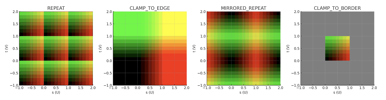
Fig. 139 Texture Warpping
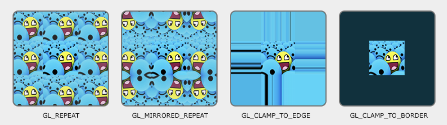
Convert normalized texture coordinates into actual memory addresses.
Texture Fetching
Retrieve texels (texture elements) from texture memory (L1 texture cache, then L2/VRAM on miss).
Handle different texture layouts: - 1D, 2D, 3D textures - Cubemaps - Texture arrays
Support compressed texture formats (e.g., DXT, ASTC, ETC2).
Texture Filtering
Give a Texture coordinates, OpenGL has to figure out which texture pixel (also known as a texel) to map the texture coordinate to.
Perform interpolation between texels to produce smooth visual results.
Filtering requires multiple texel reads + weighted average calculations.
Common filtering modes as the following are shown as Fig. 143:
Nearest-neighbor (point sampling) (GL_NEAREST)
Bilinear (GL_LINEAR)
Trilinear (with mipmaps)
Anisotropic filtering (for angled surfaces)
Let’s see how these methods work when using a texture with a low resolution on a large object (texture is therefore scaled upwards and individual texels are noticeable). The GL_NEAREST and GL_LINEAR as the following Fig. 143. As result, GL_LINEAR produces a more blurred color and smooth edge’s output.
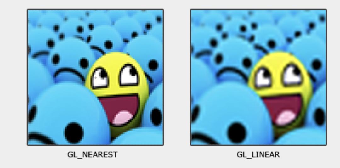
Fig. 143 Texture Filter: GL_NEAREST has sharp color and jagged edge [72]
Mipmap Level of Detail (LOD) Selection
Choose the correct mipmap level based on screen-space derivatives of texture coordinates.
Prevent aliasing and improve cache efficiency.
Optionally blend between mip levels for trilinear filtering.
Texture Caching
TMUs have a dedicated texture cache optimized for 2D/3D spatial locality.
Neighboring threads in a Warp often fetch adjacent texels, improving cache hits.
Caches reduce memory latency and improve bandwidth utilization.
Specialized Operations
Texture gather: fetch 4 neighboring texels around a coordinate.
Shadow mapping: compare fetched depth texel against reference value.
Multisample textures: fetch per-sample data for MSAA.
Border color application for out-of-bounds accesses.
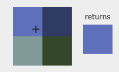

Microarchitecture Aspects
Each Streaming Multiprocessor (SM) or Compute Unit (CU) is paired with several TMUs.
The number of TMUs is a key spec in GPU datasheets (e.g., “64 TMUs”).
TMU throughput is often measured in texels per clock cycle.
Modern GPUs balance TMUs per ALU to ensure shading and texture workloads are not bottlenecked.
Performance Considerations
Bandwidth-limited: TMUs rely heavily on memory bandwidth. Mipmapping and caches reduce this pressure.
Latency hiding: texture fetches may take hundreds of cycles, so GPUs rely on massive multithreading to hide stalls.
Workload dependent: texture-heavy games or rendering pipelines are often limited by TMU throughput.
Summary
TMUs are highly specialized GPU units that:
Translate texture coordinates into addresses.
Fetch texels efficiently with dedicated caches.
Perform filtering and LOD computations in hardware.
Deliver high throughput for texture operations that are essential in realistic rendering.
Without TMUs, all these operations would fall on general-purpose ALUs, resulting in drastically lower performance and efficiency.
Render Output Units (ROPs) [111]
Function:
Processed Fragments → Pixels
Overview
Render Output Units (ROPs), also known as Raster Operations Pipelines, are the final stage in the GPU graphics pipeline before pixel data is written to the framebuffer. ROPs handle pixel-level operations such as blending, depth and stencil testing, multisample resolve, and writing to memory. They are crucial for assembling the final image that appears on screen.
Pipeline Responsibilities
Fragment Reception: Accepts shaded fragments from the pixel shader.
Depth and Stencil Testing: Compares fragment depth/stencil values against buffers.
Blending: Combines fragment color with existing framebuffer data.
Multisample Resolve: Merges multiple samples into a final pixel (for MSAA).
Framebuffer Write: Commits final pixel data to memory for display.
The pipeline flow is shown as Fig. 144.
![digraph RenderOutputPipeline {
rankdir=LR;
node [shape=box, style=filled, fillcolor=lightgray];
FragmentShader -> ROP_Unit;
ROP_Unit -> DepthStencilTest;
DepthStencilTest -> Blending;
Blending -> MSAAResolve;
MSAAResolve -> FramebufferWrite;
ROP_Unit [label="ROP Unit", fillcolor=lightyellow];
FramebufferWrite [label="Framebuffer Write", fillcolor=lightblue];
}](_images/graphviz-0ca2a2f0f8a04076216e8e204670460ef2b3fc1c.png)
Fig. 144 The pipeline for Render Output Units (ROPs)
Performance Considerations
ROP Count: More ROPs can increase pixel throughput, especially at high resolutions.
Memory Bandwidth: ROPs are tightly coupled with memory controllers; bandwidth limits can bottleneck performance.
Antialiasing Support: Hardware MSAA and resolve operations are often implemented in ROPs.
Compression: Some GPUs use framebuffer compression to reduce bandwidth usage.
Vendor-Specific Notes
NVIDIA: Refers to these units as ROPs; tightly integrated with memory partitions.
AMD: Calls them Render Backends (RBs); RDNA architecture decouples ROPs from shader engines.
Intel & ARM: Implement simplified ROPs for power-efficient mobile rendering.
References
System Features – Buffers
CPU and GPU provides different Buffers to speedup OpenGL pipeline rendering [48].
Buffer Type |
Access |
Location |
API/Usage |
Function |
Description |
|---|---|---|---|---|---|
Vertex Buffer (VBO) |
Read |
GPU |
OpenGL, Vulkan |
Store vertex attributes |
Holds data like position, normal, and texture coords for drawing geometry. |
Index Buffer (IBO/EBO) |
Read |
GPU |
OpenGL, Vulkan |
Reuse vertex data |
Stores indices into the vertex buffer to avoid duplication. |
Uniform Buffer (UBO) |
Read |
GPU or Shared |
OpenGL, Vulkan |
Constant input data |
Shares transformation matrices, lighting, or material data across shaders. |
Shader Storage Buffer (SSBO) |
Read/Write |
GPU or Shared |
OpenGL, Vulkan |
General data exchange |
Flexible, large buffers accessible for structured shader I/O. |
Constant Buffer |
Read |
GPU or Shared |
DirectX, Vulkan |
Fast uniform access |
Optimized for fast access to frequently read small data. |
Image / Texture Buffer |
Read/Write |
GPU |
OpenGL, Vulkan |
Sample/store pixels |
Stores image data for sampling or read/write image operations in shaders. |
Color Buffer |
Write |
GPU |
OpenGL, Vulkan |
Store final pixel color |
Stores output of fragment shaders; used for display or post-processing. |
Depth Buffer (Z-Buffer) |
Write/Read |
GPU |
OpenGL, Vulkan |
Visibility testing |
Stores per-pixel depth values for hidden surface removal. |
Frame Buffer |
Write |
GPU |
OpenGL, Vulkan |
Store render output |
Holds final color, depth, or other rendered output. |
Stencil Buffer |
Read/Write |
GPU |
OpenGL, Vulkan |
Pixel masking |
Used to conditionally discard or preserve pixels in the pipeline. |
Color buffer
They contain the RGB or sRGB color data and may also contain alpha values for each pixel in the framebuffer. There may be multiple color buffers in a framebuffer. You’ve already used double buffering for animation. Double buffering is done by making the main color buffer have two parts: a front buffer that’s displayed in your window; and a back buffer, which is where you render the new image [84].
Depth buffer (Z buffer)
Depth is measured in terms of distance to the eye, so pixels with larger depth-buffer values are overwritten by pixels with smaller values [85] [87] [88].
Frame Buffer
OpenGL offers: the color, depth and stencil buffers. This combination of buffers is known as the default framebuffer and as you’ve seen, a framebuffer is an area in memory that can be rendered to [90].
Stencil Buffer
In the simplest case, the stencil buffer is used to limit the area of rendering (stenciling) [89] [88].
Buffer Type |
Access |
Location |
API/Usage |
Function |
Description |
|---|---|---|---|---|---|
Compute Buffer |
Read/Write |
GPU or Shared |
OpenCL, Vulkan, CUDA |
Parallel compute data |
Buffers used in compute kernels or shaders for general processing. |
Atomic Buffer |
Read/Write (Atomic) |
GPU |
OpenGL, Vulkan |
Shared counters/data |
Used with atomic ops for synchronization or accumulation. |
Acceleration Structure Buffer |
Read |
GPU |
Vulkan RT, DXR |
Ray tracing acceleration |
Holds spatial hierarchy (BVH) for ray traversal efficiency. |
Indirect Draw Buffer |
Read |
GPU |
Vulkan, DirectX |
GPU-issued draw |
Stores draw/dispatch args to issue commands without CPU. |
DXR: DirectX Raytracing — a D3D12 extension for real-time ray tracing using GPU acceleration.
Indirect Draw Buffer: A GPU-side buffer holding draw parameters so that GPU (not CPU) can issue rendering work dynamically.
Buffer Type |
Access |
Location |
API/Usage |
Function |
Description |
|---|---|---|---|---|---|
Command Buffer |
Write (CPU) / Read (GPU) |
Host → GPU |
Vulkan, DirectX12 |
Submit work |
Encapsulates commands like draw, dispatch, and memory ops. |
Parking / Staging Buffer |
Read/Write |
Host-visible |
Vulkan, CUDA |
Temporary transfer |
Temporary CPU-visible buffer for uploading/downloading GPU data. |
Software Structure
As the previous section illustrated, GPU is a SIMT (SIMD) for data parallel application. This section introduces the GPU evolved from Graphics GPU to the General purpose GPU (GPGPU) and the software architecture of GPUs and explores AI software frameworks designed for GPUs, NPUs, and CPUs.
General purpose GPU
Since GLSL shaders provide a general way for writing C code in them, if applying a software frame work instead of OpenGL API, then the system can run some data parallel computation on GPU for speeding up and even get CPU and GPU executing simultaneously. Furthmore, any language that allows the code running on the CPU to poll a GPU shader for return values, can create a GPGPU framework [91].
Mapping data in GPU
As described in the previous section on GPUs, the subset of the array calculation y[] = a * x[] + y[] is shown as follows:
// Invoke DAXPY with 256 threads per Thread Block
__host__
int nblocks = (n+255) / 256;
daxpy<<<nblocks, 256>>>(n, 2.0, x, y);
// DAXPY in CUDA
__device__
void daxpy(int n, double a, double *x, double *y) {
  int i = blockIdx.x*blockDim.x + threadIdx.x;
  if (i < n) y[i] = a*x[i] + y[i];
}
name<<<dimGrid, dimBlock>>>(… parameter list …):
dimGrid: Number of Blocks in Grid
dimBlock: 256 Threads in Block
Assembly code of PTX (from page 300 of Quantitative book)
// code to set VLR, Vector Length Register, to (n % 256)
//   ...
//
shl.u32 R8, blockIdx, 9       ; Thread Block ID * Block size (512)
add.u32 R8, R8, threadIdx     ; R8 = i = my CUDA Thread ID
shl.u32 R8, R8, 3             ; byte offset
setp.neq.s32 P1, RD8, RD3     ; RD3 = n, P1 is predicate register 1
ld.global.f64 RD0, [X+R8]     ; RD0 = X[i]
ld.global.f64 RD2, [Y+R8]     ; RD2 = Y[i]
mul.f64 RD0, RD0, RD4         ; Product in RD0 = RD0 * RD4 (scalar a)
add.f64 RD0, RD0, RD2         ; SuminRD0 = RD0 + RD2 (Y[i])
st.global.f64 [Y+R8], RD0     ; Y[i] = sum (X[i]*a + Y[i])
Need to set VLR if PTX has this instruction. Otherwise, set lane-mask in the similar way of the code below.
__device__
void lane-mask-ex( double *X, double *Y, double *Z) {
  if (X[i] != 0)
    X[i] = X[i] – Y[i];
  else X[i] = Z[i];
}
Assembly code of Vector Processor
LV V1,Rx         ;load vector X into V1
LV V2,Ry         ;load vector Y
L.D F0,#0        ;load FP zero into F0
SNEVS.D V1,F0    ;sets VM(i) to 1 if V1(i)!=F0
SUBVV.D V1,V1,V2 ;subtract under vector mask
SV V1,Rx         ;store the result in X
Assembly code of PTX (modified code from refering page 208 - 302 of Quantitative book)
ld.global.f64 RD0, [X+R9]     ; RD0 = X[i]
setp.neq.s32 P1, RD0, #0      ; P1 is predicate register 1
@!P1, bra ELSE1, *Push        ; Push old mask, set new mask bits
                              ; if P1 false, go to ELSE1
ld.global.f64 RD2, [Y+R8]     ; RD2 = Y[i]
sub.f64 RD0, RD0, RD2         ; Difference in RD0
st.global.f64 [X+R8], RD0     ; X[i]=RD0
ELSE1:
ld.global.f64 RD0, [Z+R8]     ; RD0 = Z[i]
st.global.f64 [X+R8], RD0     ; X[i] = RD0
ENDIF1:
ret, *Pop                     ; pop to restore old mask
The following table explains how the elements of saxpy() are mapped to the Lanes of a SIMD Thread (Warp), which belongs to a Thread Block (Core) within a Grid.
saxpy(() |
Instance in Fig. 127 |
Description |
|---|---|---|
blockDim.x |
The index of Thread Block |
blockDim: in this example configured as Fig. 127 is 16(Thread Blocks) * 16(SIDM Threads) = 256 |
blockIdx.x |
The index of SIMD Thread |
blockIdx: the index of Thread Block within the Grid |
threadIdx.x |
The index of elements |
threadIdx: the index of the SIMD Thread within its Thread Block |
With Fermi, each 32-wide thread of SIMD instructions is mapped to 16 physical SIMD Lanes, so each SIMD instruction in a thread of SIMD instructions takes two clock cycles to complete.
You could say that it has 16 Lanes, the vector length would be 32, and the Chime is 2 clock cycles.
The mape of y[0..31] = a * x[0..31] * y[0..31] to <Core, Warp, Cuda Thread> of GPU as the following table. x[0..31] map to 32 Cuda Threads; two Cuda Threads map to one SIMD Lane as Fig. 126..
Warp-0 |
Warp-1 |
… |
Warp-15 |
|
|---|---|---|---|---|
Core-0 |
y[0..31] = a * x[0..31] * y[0..31] |
y[32..63] = a * x[32..63] + y[32..63] |
… |
y[480..511] = a * x[480..511] + y[480..511] |
… |
… |
… |
… |
… |
Core-15 |
y[7680..7711] = a * … |
… |
… |
y[8160..8191] = a * x[8160..8191] + y[8160..8191] |
Each Cuda Thread runs the GPU function code saxpy. Fermi has a register file of size 32768 x 32-bit. As shown in Fig. 118, the number of registers in a Thread Block is: 16 (SM) * 32 (Cuda Threads) * 64 (TLR, Thread Level Register) = 32768 x 32-bit (Register file).
When mapping to fragments/pixels in a graphics GPU, x[0..15] corresponds to a two-dimensional tile of fragments/pixels at pixel[0..3][0..3], since images use tile-based grouping to cluster similar colors together.
Work between CPU and GPU in Cuda
The previous daxpy() GPU code did not include the host (CPU) side code that triggers the GPU function.
The following example shows the host (CPU) side of a CUDA program that calls saxpy on the GPU [94]:
#include <stdio.h>

__global__
void saxpy(int n, float a, float * x, float * y)
{
  int i = blockIdx.x*blockDim.x + threadIdx.x;
  if (i < n) y[i] = a*x[i] + y[i];
}

int main(void)
{
  ...
  cudaMemcpy(d_x, x, N*sizeof(float), cudaMemcpyHostToDevice);
  cudaMemcpy(d_y, y, N*sizeof(float), cudaMemcpyHostToDevice);
  ...
  saxpy<<<(N+255)/256, 256>>>(N, 2.0, d_x, d_y);
  ...
  cudaMemcpy(y, d_y, N*sizeof(float), cudaMemcpyDeviceToHost);
  ...
}
The main() function runs on the CPU, while saxpy() runs on the GPU. The CPU copies data from x and y to the corresponding device arrays d_x and d_y using cudaMemcpy.
The saxpy kernel is launched with the following statement:
saxpy<<<(N+255)/256, 256>>>(N, 2.0, d_x, d_y);
This launches the kernel with Thread Blocks containing 256 threads, and uses integer arithmetic to determine the number of Thread Blocks needed to process all N elements in the arrays. The expression (N+255)/256 ensures full coverage of the input data.
Using cudaMemcpyHostToDevice and cudaMemcpyDeviceToHost, the CPU can pass data in x and y to the GPU, and retrieve the results back to y.
Since both memory transfers are handled by DMA and do not require CPU operation, the performance can be improved by running CPU and GPU independently, each accessing their own cache.
After the DMA copy from CPU memory to GPU memory, the GPU performs the full matrix operation loop for y[] = a * x[] + y[]; using a single Grid of threads.
DMA memcpy maps the data in CPU memory to each L1 cache of a core on GPU memory.
Many GPUs support scatter and gather operations to access DRAM efficiently for stream processing tasks [106] [91] [107].
When the GPU function is dense computation in array such as MPEG4 encoder or deep learning for tuning weights, it may get much speed up [108]. However when GPU function is matrix addition and CPU will idle for waiting GPU’s result. It may slow down than doing matrix addition by CPU only. Arithmetic intensity is defined as the number of operations performed per word of memory transferred. It is important for GPGPU applications to have high arithmetic intensity else the memory access latency will limit computational speedup [91].
Wiki here [109] includes GPU-accelerated applications for speedup as follows:
General Purpose Computing on GPU, has found its way into fields as diverse as machine learning, oil exploration, scientific image processing, linear algebra, statistics, 3D reconstruction and even stock options pricing determination. In addition, section “GPU accelerated video decoding and encoding” for video compressing [109] gives the more applications for GPU acceleration.
Item |
CPU |
GPU |
|---|---|---|
Application |
Non-data parallel |
Data parallel |
Architecture |
SISD, small vector (eg.4*32bits) |
Large SIMD (eg.16*32bits) |
Cache |
Smaller and faster |
Larger and slower (ref. The following Note) |
ILP |
Pipeline |
Pipeline |
Superscalar, SMT |
SIMT |
|
Super-pipeline |
||
Core |
Smaller threads for SMT (2 or 4) |
Larger threads (16 or 32) |
Branch |
Conditional-instructions |
Mask & conditional-instructions |
Note
GPU-Cache
In theory, for data-parallel applications using GPU’s SMT, the GPU can schedule more threads and aims for throughput rather than speedup of a single thread, as seen in SISD on CPUs.
However, in practice, GPUs provide only a small L1 cache, similar to CPUs, and handle cache misses by scheduling another thread.
As a result, GPUs often lack L2 and L3 caches, which are common in CPUs with deeper cache hierarchies.
OpenCL, Vulkan and spir-v
![digraph G {
rankdir=LR;
compound=true;
node [shape=record];
SW_LAYER [label="{ GLSL | OpenCL } | SPIR-V | GPU machine code"];
}](_images/graphviz-2bc5c5193c3ea5662118149e273bcb3969bcc50c.png)
Fig. 145 OpenCL and GLSL(OpenGL)
Name of SW |
GPU language |
Level of GPU language |
|---|---|---|
OpenCL |
OpenCL |
C99 dialect (with C pointer, …) |
OpenGL |
GLSL |
C-like (no C pointer, …) |
Vulkan |
SPIR-V |
IR |
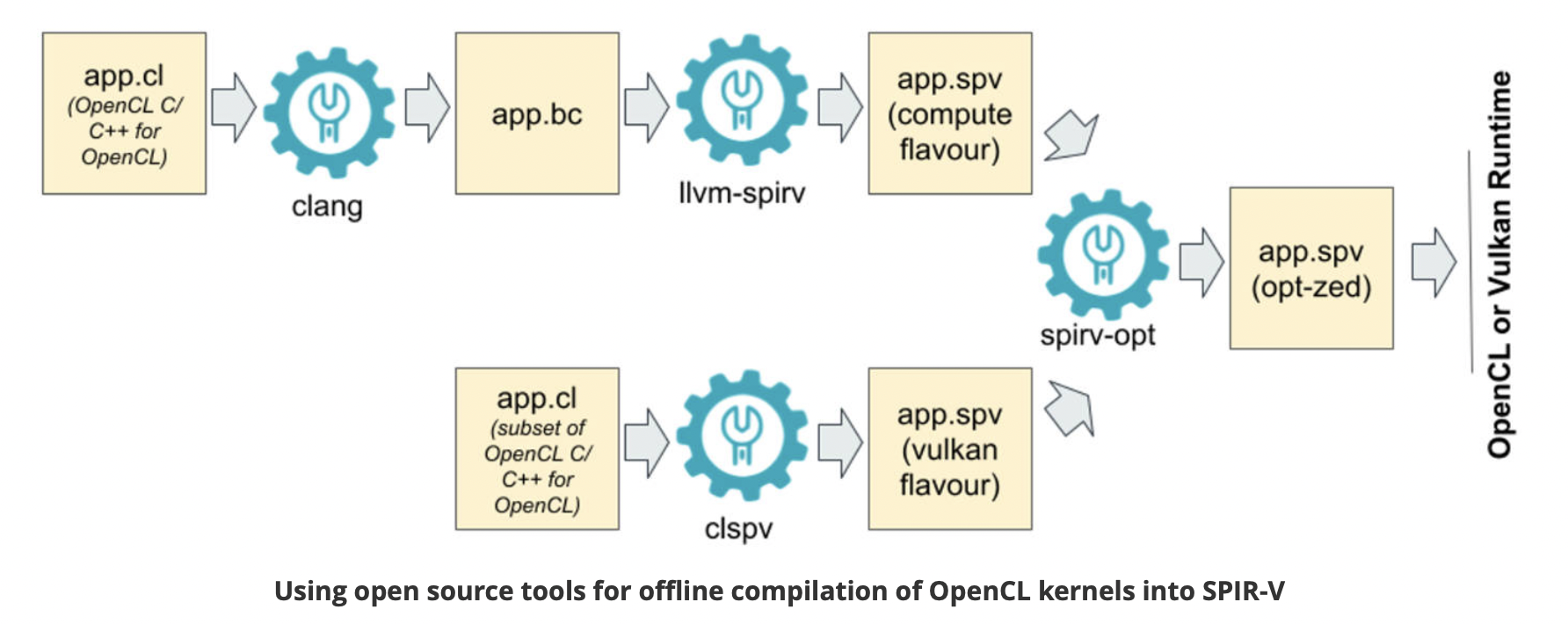
Fig. 146 Offline Compilation of OpenCL Kernels into SPIR-V Using Open Source Tooling [113]
clang: Compile OpenCL to spirv for runtime+driver. Or compile OpenCL to llvm, then “SPIR-V LLVM Translator” translate llvm to spirv for runtime+driver.
clspv: Compile OpenCL to spirv directly.
![digraph ShaderToLLVMIR {
rankdir=LR;
node [shape=record, style=filled, color=black];
// Source Languages
GLSL [label="GLSL ES (OpenGL)", fillcolor=white];
OpenCL_C [label="OpenCL C", fillcolor=white];
// Intermediate Representation
SPIRV [label="SPIR-V", fillcolor=orange];
GPU_ISA [label="GPU ISA in Assembly and Binary", fillcolor=grey];
// LLVM IR
LLVM_IR [label="LLVM IR", fillcolor=orange];
// Tools with oval shapes
node [shape=oval, style=filled, fillcolor=lightgreen];
Glslang [label="glslangValidator", fillcolor=lightblue];
CL_SPIRV [label="OpenCL-SPIRV Translator"];
// Tools with oval shapes
node [shape=oval, style=filled, fillcolor=yellow];
SPIRV_LLVM [label="SPIRV-LLVM Translator"];
LLVMCompiler [label="Backend Compiler"];
// Edges
GLSL -> Glslang -> SPIRV;
OpenCL_C -> CL_SPIRV -> SPIRV -> SPIRV_LLVM -> LLVM_IR -> LLVMCompiler -> GPU_ISA;
}](_images/graphviz-eaa1c1adef57f7a08f883ff241a92b8badf1ea7a.png)
Fig. 147 GPU Compiler Components and Flow
The flow and relationships among GLSL, OpenCL, SPIR-V (Vulkan/OpenCL), LLVM IR, and the GPU compiler are shown in the Fig. 145, Fig. 146 and Fig. 147. As shown in Fig. 147, OpenCL-C to SPIR-V (OpenCL) can be compiled using clang + llvm-spirv tools or a proprietary converter.
As shown in Fig. 147, both GLSL and OpenCL use frontend tools to generate SPIR-V. The driver can invoke either the GLSL or OpenCL compiler based on metadata fields in the SPIR-V, as illustrated in Fig. 148 and the following figures, which describe offline compilation from GLSL/OpenCL to SPIR-V and online execution using the generated SPIR-V files.
![digraph SPIRV_Deployment {
rankdir=LR;
node [shape=box, style=filled, fillcolor=lightgray, fontname="Helvetica"];
subgraph cluster_glsl {
label = "From GLSL";
glsl_src [label="GLSL Shader\n (.vert/.frag/.comp)", fillcolor=lightblue];
glsl_compiler [label="glslangValidator\n(or similar compiler)", fillcolor=lightgreen];
spirv_glsl [label="SPIR-V\n (from GLSL)", fillcolor=gold];
glsl_src -> glsl_compiler -> spirv_glsl;
}
subgraph cluster_opencl {
label = "From OpenCL C";
opencl_src [label="OpenCL C (.cl)", fillcolor=lightblue];
clang_spirv [label="Clang + SPIR-V Backend", fillcolor=lightgreen];
spirv_opencl [label="SPIR-V\n (from OpenCL C)", fillcolor=gold];
opencl_src -> clang_spirv -> spirv_opencl;
}
subgraph cluster_opencl_runtime {
label = "OpenCL Runtime (Host)";
spirv_loader [label="clCreateProgramWithIL()", fillcolor=orange];
spirv_glsl -> spirv_loader;
spirv_opencl -> spirv_loader;
spirv_loader -> device_driver [label="Load\n SPIR-V\n into driver"];
device_driver [label="OpenCL Driver\n(SPIR-V → Device IR → Machine Code)", fillcolor=plum];
device_driver -> execution [label="Compiled &\n Run on device"];
execution [label="Execute on\n OpenCL Device", fillcolor=lightyellow];
}
// Styling
edge [fontname="Helvetica"];
}](_images/graphviz-2bc7461ac50af10b847453fe0da75d1a3ddf5bf7.png)
Fig. 148 Compiling and Deploying GPU Code from GLSL, Vulkan, and OpenCL
Based on the flows above, the public standards OpenGL and OpenCL provide tools for transferring these data format, as illustrated in Fig. 149. The corresponding LLVM IR and SPIR-V formats are listed below.
![digraph G {
rankdir=LR;
// Data Nodes
node [shape=record, style=filled, fillcolor=white];
glsl [label="glsl"];
openclc [label="OpenCL C"];
spirv [label="spirv"];
llvm [label="llvm-ir"];
// Tools Nodes
node [shape=oval, style=filled, fillcolor=lightgreen];
glslang [label="glslangValidator"];
spirv_cross [label="spirv-cross"];
clspv [label="clspv"];
llvm_spirv [label="llvm-spirv"];
glsl -> glslang -> spirv;
glsl -> spirv_cross -> spirv [dir="back"];
openclc -> clspv -> spirv;
openclc -> clspv -> spirv [dir="back"];
spirv -> llvm_spirv -> llvm;
llvm -> llvm_spirv -> spirv;
}](_images/graphviz-e76f03aa0cacc2b0edb5a70fc6147e5f3dbd12fa.png)
Fig. 149 Convertion between GLSL, OpenCL C, SPIRV-V and LLVM-IR
References/add-matrix.ll
; ModuleID = 'add-matrix.ll'
target datalayout = "e-p:64:64:64-i1:8:8-i8:8:8-i16:16:16-i32:32:32-i64:64:64-f32:32:32-f64:64:64-v16:16:16-v24:32:32-v32:32:32-v48:64:64-v64:64:64-v96:128:128-v128:128:128-v192:256:256-v256:256:256-v512:512:512-v1024:1024:1024-G1"
target triple = "spir64-unknown-unknown"

; Function Attrs: nounwind
define spir_func <4 x i32> @add_mat(<4 x i32> %a, <4 x i32> %b) #0 {
entry:
  %sum = add <4 x i32> %a, %b
  ret <4 x i32> %sum
}

attributes #0 = { nounwind }

!spirv.MemoryModel = !{!0}
!opencl.enable.FP_CONTRACT = !{}
!spirv.Source = !{!1}
!opencl.spir.version = !{!2}
!opencl.used.extensions = !{!3}
!opencl.used.optional.core.features = !{!3}
!spirv.Generator = !{!4}

!0 = !{i32 2, i32 2}
!1 = !{i32 0, i32 0}
!2 = !{i32 1, i32 2}
!3 = !{}
!4 = !{i16 6, i16 14}
References/add-matrix.spvasm
; SPIR-V
; Version: 1.0
; Generator: Khronos LLVM/SPIR-V Translator; 14
; Bound: 10
; Schema: 0
               OpCapability Addresses
               OpCapability Linkage
               OpCapability Kernel
          %1 = OpExtInstImport "OpenCL.std"
               OpMemoryModel Physical64 OpenCL
               OpSource Unknown 0
               OpName %add_mat "add_mat"
               OpName %a "a"
               OpName %b "b"
               OpName %entry "entry"
               OpName %sum "sum"
               OpDecorate %add_mat LinkageAttributes "add_mat" Export
       %uint = OpTypeInt 32 0
     %v4uint = OpTypeVector %uint 4
          %4 = OpTypeFunction %v4uint %v4uint %v4uint
    %add_mat = OpFunction %v4uint None %4
          %a = OpFunctionParameter %v4uint
          %b = OpFunctionParameter %v4uint
      %entry = OpLabel
        %sum = OpIAdd %v4uint %a %b
               OpReturnValue %sum
               OpFunctionEnd
Convert between spirv and llvm-ir
% pwd
$HOME/git/lbd/References
% llvm-as -o add-matrix.bc add-matrix.ll
% llvm-spirv -o add-matrix.spv add-matrix.bc
% spirv-dis -o add-matrix.spvasm add-matrix.spv
// Convert spirv to llvm-ir again and check the converted llvm-ir is same
// with origin.
% llvm-spirv -r add-matrix.spv -o add-matrix.spv.bc
% llvm-dis add-matrix.spv.bc -o add-matrix.spv.bc.ll
% diff add-matrix.ll add-matrix.spv.bc.ll
1c1
< ; ModuleID = 'add-matrix.ll'
---
> ; ModuleID = 'add-matrix.spv.bc'
Install llvm-spriv and llvm with Brew-install
% brew install spirv-llvm-translator
% brew install llvm
The following explains how the driver identifies whether the SPIR-V source is from GLSL or OpenCL.
SPIR-V binaries contain metadata that can help identify whether they were generated from OpenCL, GLSL, or another language.
Execution Model
Defined by the OpEntryPoint instruction. It is a strong indicator of the source language.
ExecutionModel
Typical Source
Notes
Kernel
OpenCL
Used only by OpenCL C
GLCompute
GLSL or HLSL
Used in compute shaders
Fragment
GLSL or HLSL
For pixel shaders
Vertex
GLSL or HLSL
For vertex shaders
Capabilities
Declared using OpCapability. They provide clues about the SPIR-V’s execution model and source.
Capability
Likely Source
Kernel
OpenCL
Addresses
OpenCL
Linkage
OpenCL
Shader
GLSL or HLSL
Extensions
Declared using OpExtension. Some are tied to specific compilers or languages.
Extension
Likely Source
SPV_KHR_no_integer_wrap_decoration
OpenCL
SPV_INTEL_unified_shared_memory
OpenCL (Intel)
SPV_AMD_shader_ballot
GLSL (graphics)
Memory Model
Defined by OpMemoryModel.
OpenCL → OpenCL source
GLSL450 → GLSL or HLSL source
How to Inspect
Use the spirv-dis tool to disassemble SPIR-V to human-readable form:
spirv-dis kernel.spv -o kernel.spvasm
Look for these at the top of the file:
Example (GLSL):
OpCapability Shader
OpMemoryModel Logical GLSL450
OpEntryPoint GLCompute %main "main"
Example (OpenCL):
OpCapability Kernel
OpCapability Addresses
OpMemoryModel Logical OpenCL
OpEntryPoint Kernel %foo "foo"
Summary
Feature |
Indicates |
|---|---|
OpEntryPoint Kernel |
OpenCL |
OpCapability Shader |
GLSL or HLSL |
OpMemoryModel OpenCL |
OpenCL |
OpMemoryModel GLSL450 |
GLSL or HLSL |
Comparsion for OpenCL and OpenGL’s compute shader.
Same:
Both are for General Computing of GPU.
Difference:
OpenCL include GPU and other accelerate device/processor. OpenCL is C language on Device and C++ on Host based on OpenCL runtime. Compute shader is GLSL shader language run on OpenGL graphic enviroment and integrate and access data of OpenGL API easily [112].
OpenGL/GLSL vs Vulkan/spir-v.
High level of API and shader: OpenGL, GLSL.
Low level of API and shader: Vulkan, spir-v.
Though OpenGL api existed in higher level with many advantages from sections above, sometimes it cannot compete in efficience with direct3D providing lower levels api for operating memory by user program [114]. Vulkan api is lower level’s C/C++ api to fill the gap allowing user program to do these things in OpenGL to compete against Microsoft direct3D. Here is an example [115]. Meanwhile glsl is C-like language. The vulkan infrastructure provides tool, glslangValidator [116], to compile glsl into an Intermediate Representation Form (IR) called spir-v off-line. As a result, it saves part of compilation time from glsl to gpu instructions on-line since spir-v is an IR of level closing to llvm IR [117]. In addition, vulkan api reduces gpu drivers efforts in optimization and code generation [114]. These standards provide user programmer option to using vulkan/spir-v instead of OpenGL/glsl, and allow them pre-compiling glsl into spir-v off-line to saving part of on-line compilation time.
With vulkan and spir-v standard, the gpu can be used in OpenCL for Parallel Programming of Heterogeneous Systems [118] [119]. Similar with Cuda, a OpenCL example for fast Fourier transform (FFT) is here [120]. Once OpenCL grows into a popular standard when more computer languages or framework supporting OpenCL language, GPU will take more jobs from CPU [121].
Most GPUs have 16 or 32 Lanes in a SIMD processor (Warp), vulkan provides Subgroup operations to data parallel programming on Lanes of SIMD processor [122].
Subgroup operations provide a fast way for moving data between Lanes intra Warp. Assuming each Warp has eight Lanes. The following table lists result of reduce, inclusive and exclusive operations.
Lane |
0 |
1 |
2 |
3 |
|---|---|---|---|---|
Initial value |
a |
b |
c |
d |
Reduce |
OP(abcd) |
OP(abcd) |
OP(abcd) |
OP(abcd) |
Inclusive |
OP(a) |
OP(ab) |
OP(abc) |
OP(abcd) |
Exclusive |
not define |
OP(a) |
OP(ab) |
OP(abc) |
Reduce: e.g. subgroupAdd. Inclusive: e.g. subgroupInclusiveAdd. Exclusive: e.g. subgroupExclusiveAdd.
For examples:
ADD operation: OP(abcd) = a+b+c+d.
MAX operation: OP(abc) = MAX(a,b,c).
When Lane i is inactive, it is value is none.
For instance of Lane 0 is inactive, then MUL operation: OP(abcd) = b*c*d.
The following is a code example.
An example of subgroup operations in glsl for vulkan
vec4 sum = vec4(0, 0, 0, 0);
if (gl_SubgroupInvocationID < 16u) {
  sum += subgroupAdd(in[gl_SubgroupInvocationID]);
}
else {
  sum += subgroupInclusiveMul(in[gl_SubgroupInvocationID]);
}
subgroupMemoryBarrier();
Nvidia’s GPU provides __syncWarp() for subgroupMemoryBarrier() or compiler to sync for the Lanes in the same Warp.
In order to let Lanes in the same SIMD processor work efficently, data unifomity analysis will provide many optimization opporturnities in register allocation, transformation and code generation [123].
LLVM IR expansion from CPU to GPU is becoming increasingly influential. In fact, LLVM IR has been expanding steadily from version 3.1 until now, as I have observed.
Unified IR Conversion Flows
Graphics and OpenCL Compilation
This section outlines the intermediate representation (IR) flows for graphics (Microsoft DirectX, OpenGL) and OpenCL compilation across major GPU vendors: NVIDIA, AMD, ARM, Imagination Technologies, and Apple.
Graphics Compilation Flow (Microsoft DirectX & OpenGL)
Graphics shaders are compiled from high-level languages (HLSL, GLSL) into vendor-specific GPU binaries via intermediate representations like DXIL and SPIR-V.
✅ Each node in the graph is color-coded to indicate its category or role within the structure.
![digraph G {
node [shape=box, style=filled];
PUIR [label="Public standard of IRs", fillcolor=lightyellow];
PRIR [label="Private IRs", fillcolor=lightgray];
VD [label="Vendor Driver", shape=oval, fillcolor=lightgreen];
GPU [label="GPU", fillcolor=lightblue];
}](_images/graphviz-a74f6bea943a022cb282ae6be819852518bafa2b.png)
Vendor Driver will call Vendor Compiler for on-line compilation.
![digraph OpenCL_OpenGL_Compilation {
rankdir=LR;
node [shape=box];
// Source Languages
OpenCL_C [style=filled, fillcolor=lightyellow];
GLSL [style=filled, fillcolor=lightyellow];
// Shared IRs
SPIR [style=filled, fillcolor=lightyellow];
SPIRV [label="SPIR-V IR", style=filled, fillcolor=lightyellow];
LLVM_IR [style=filled, fillcolor=lightyellow];
// Vendor Drivers
node [shape=oval];
"NVIDIA Driver" [style=filled, fillcolor=lightgreen];
"AMD Driver" [style=filled, fillcolor=lightgreen];
"ARM Driver" [style=filled, fillcolor=lightgreen];
"Imagination Driver" [style=filled, fillcolor=lightgreen];
"Apple Driver" [style=filled, fillcolor=lightgreen];
// Private IRs
node [shape=box];
"PTX IR" [style=filled, fillcolor=gray];
"GCN IR" [style=filled, fillcolor=gray];
"Burst IR" [style=filled, fillcolor=gray];
"Metal IR" [style=filled, fillcolor=gray];
// GPU Targets
"NVIDIA GPU ISA" [style=filled, fillcolor=lightblue];
"AMD GPU ISA" [style=filled, fillcolor=lightblue];
"ARM Mali ISA" [style=filled, fillcolor=lightblue];
"Imagination USC ISA" [style=filled, fillcolor=lightblue];
"Apple GPU ISA" [style=filled, fillcolor=lightblue];
// OpenCL Flow
OpenCL_C -> SPIR -> LLVM_IR;
OpenCL_C -> SPIRV;
// OpenGL Flow
GLSL -> SPIRV -> LLVM_IR;
// LLVM based Compilation Flow
LLVM_IR -> "PTX IR" -> "NVIDIA Driver" -> "NVIDIA GPU ISA";
LLVM_IR -> "GCN IR" -> "AMD Driver" -> "AMD GPU ISA";
LLVM_IR -> "ARM Driver" -> "ARM Mali ISA";
LLVM_IR -> "Burst IR" -> "Imagination Driver" -> "Imagination USC ISA";
LLVM_IR -> "Metal IR" -> "Apple Driver" -> "Apple GPU ISA";
}](_images/graphviz-f31784f2c1cea659a3c6e4c51e4c5a3c00dee795.png)
Fig. 150 Graphics and OpenCL Compiler IR Conversion Flow
OpenCL C is the device side code in C language while Host side code is C/C++.
OpenCL C is compiled to SPIR-V in later versions of OpenCL, while earlier versions used SPIR. SPIR-V has now largely replaced SPIR as the standard intermediate representation.
IR Layer |
Abstraction Level |
Register Model |
|---|---|---|
PTX (NVIDIA) |
Virtual ISA; portable across GPU generations; hides hardware scheduling |
Virtual registers (%r, %f); mapped to physical registers during SASS lowering |
GCN IR (AMD) |
Machine IR; tightly coupled to GCN/RDNA architecture; exposes Wavefront semantics |
Explicit vector (vN) and scalar (sN) registers; register pressure affects occupancy. AMD’s compiler backend can lower vector operations to scalar instructions on low-end GPUs, while preserving vector operations on high-end architectures. |
Burst IR (Imagination) |
Power-aware IR; optimized for burst-core scheduling and latency hiding |
Operand staging model; abstracted register usage; mapped late to USC ISA |
Metal IR (Apple) |
LLVM-inspired IR; abstracted from developers; tuned for tile shading and threadgroup fusion |
Region-based register allocation; dynamic renaming; not exposed as physical register model |
- ✅ NVIDIA, AMD, ARM and Imagination all have exposed LLVM IR and convert SPIR-V IR to LLVM IR.
SPIR:
For OpenCL development, the IR started from SPIR (LLVM-based IR).
SPIRV’s Limitation: tightly coupled to specific LLVM versions, making it brittle across.
SPIR-V:
A complete redesign: binary format, not tied to LLVM.
Designed for Vulkan, but also supports OpenCL and OpenGL.
Enables cross-vendor portability, shader reflection, and custom extensions.
Used in graphics and compute pipelines, including ML workloads via Vulkan compute.
A Vulkan shader written in GLSL is compiled to SPIR-V, then passed to the GPU driver.
An OpenCL kernel written in C can be compiled to SPIR-V, then lowered to LLVM IR internally by vendors like AMD or NVIDIA.
⚠️ Apple
Uses LLVM IR Partially. Apple supports SPIR-V in Metal and OpenCL, but LLVM IR is not always exposed.
Metal shaders are compiled via MetalIR, which is LLVM-inspired but not standard LLVM IR. Metal IR is not standard LLVM IR and is not exposed to developers.
Apple’s ML compiler stack may use LLVM IR internally, but it’s abstracted from developers.
Apple is not a vendor of GPU IP, so it does not expose LLVM IR in its ML or graphics APIs for the reasons below:
Security: opaque compilation prevents tampering
Performance tuning: Apple controls the entire stack for optimal hardware use
Developer simplicity: high-level APIs reduce friction
Notes:
HLSL → DXIL → DirectX is Microsoft’s graphics pipeline, used on Windows and Xbox.
GLSL → SPIR-V → OpenGL/Vulkan is cross-platform and supported by all vendors.
Final GPU ISA varies by vendor:
NVIDIA: PTX → SASS
AMD: LLVM IR → GCN/RDNA
ARM: Mali ISA
Imagination: USC ISA
Apple: Metal GPU ISA
Notes:
OpenCL C → SPIR → Vendor Driver → GPU ISA is the standard compilation path.
Some vendors (e.g., AMD, NVIDIA) may bypass SPIR and compile directly to LLVM IR or PTX.
Apple deprecated OpenCL in favor of Metal, but legacy support remains.
References
OpenCL Specification: https://www.khronos.org/opencl/
SPIR-V Specification: https://www.khronos.org/spir
DirectX Shader Compiler: https://github.com/microsoft/DirectXShaderCompiler
Imagination E-Series GPU: https://www.imaginationtech.com/
Apple Metal API: https://developer.apple.com/metal/
ML and GPU Compilation
This section outlines the intermediate representation (IR) flows used by NVIDIA, AMD, and ARM in machine learning and GPU compilation pipelines. It includes both inference engines and compiler toolchains.
✅ Each node in the graph is color-coded to indicate its category or role within the structure. In AI, usually use runtime instead of driver for graphics.
![digraph G {
node [shape=box, style=filled];
PUIR [label="Public standard of IRs", fillcolor=lightyellow];
PRIR [label="Private IRs", fillcolor=lightgray];
VDLR [label="Vendor Driver,\nLibrary or Runtime", shape=oval, fillcolor=lightgreen];
MA [label="Machine", fillcolor=lightblue];
}](_images/graphviz-8772109fe3076546cd98705888b9aaecefb3e1aa.png)
NVIDIA IR Conversion Flow
NVIDIA supports both TensorRT-based inference and MLIR-based compilation targeting CUDA GPUs is shown as Fig. 151.
![digraph NVIDIA_IR_Flow {
rankdir=LR;
node [shape=box];
ONNX [style=filled, fillcolor=lightyellow];
"TensorRT Graph IR" [style=filled, fillcolor=lightgray];
"CUDA Kernel IR" [style=filled, fillcolor=lightgray];
PTX [style=filled, fillcolor=lightyellow];
SASS [label="SASS (NVIDIA GPU ISA)", style=filled, fillcolor=lightblue];
TensorRT [style=filled, shape=oval, fillcolor=lightgreen];
TOSA [style=filled, fillcolor=lightyellow];
"MLIR GPU Dialects" [style=filled, fillcolor=lightyellow];
"LLVM IR" [style=filled, fillcolor=lightyellow];
ONNX -> "TensorRT Graph IR" -> "CUDA Kernel IR" -> PTX;
"TensorRT Graph IR" -> TensorRT;
TOSA -> "MLIR GPU Dialects" -> "LLVM IR" -> PTX -> SASS;
}](_images/graphviz-f0d821a0d32e00e60d167a124e2cd0b597d45b93.png)
Fig. 151 NVIDIA IR Conversion Flow
SASS stands for Streaming ASSembler, and it represents the native instruction set architecture (ISA) for NVIDIA GPUs.
TensorRT is a C++ library and runtime developed by NVIDIA for deep learning inference—the phase where trained models make predictions.
CUDA Kernel IR is a bridge between LLVM IR and PTX/SASS, or a direct output from TensorRT.
LLVM IR is foundational in many flows, but TensorRT may skip it and directly emit CUDA kernels.
Although MLIR dialects may be publicly available, they are typically hardware-dependent and tailored to specific vendors’ GPU architectures. As a result, their applicability is limited to the corresponding hardware platforms.
MLIR GPU Dialects is public but it is for Nvidia’s GPU.
AMD IR Conversion Flow
AMD uses ROCm and MIOpen for ML workloads, with LLVM-based compilation targeting GCN or RDNA architectures is shown as Fig. 152.
![digraph ROCm_Runtime_PyTorch_MIOpen_PreMLIR_Flow {
rankdir=LR;
node [shape=box];
// Entry points
PyTorch_Model [label="PyTorch Model", style=filled, fillcolor=lightyellow];
ONNX_Model [label="ONNX Model", style=filled, fillcolor=lightyellow];
MLIR_TOSA [label="MLIR (TOSA dialect)", style=filled, fillcolor=lightyellow];
// Pre-MLIR optimization
MIOpen_PreMLIR [label="MIOpen Graph IR (Pre-MLIR)", style=filled, fillcolor=gray];
// Compilation layers
ONNX_MLIR [label="ONNX-MLIR", style=filled, fillcolor=lightyellow];
MLIR_GPU [label="MLIR GPU dialect", style=filled, fillcolor=lightyellow];
LLVM_IR [style=filled, fillcolor=lightyellow];
ROCm_BC [label="ROCm device libraries (.bc)", shape=oval, style=filled, fillcolor=lightgreen];
GCN_IR [style=filled, fillcolor=gray];
// Post-GCN optimization
MIOpen_IR [label="MIOpen Graph IR (Post-GCN)", style=filled, fillcolor=gray];
// Runtime layers
ROCr_Runtime [label="ROCr Runtime", shape=oval, style=filled, fillcolor=lightgreen];
// GPU Targets
GPU [label="AMD GPU ISA", style=filled, fillcolor=lightblue];
// Flow paths
PyTorch_Model -> ONNX_Model;
ONNX_Model -> MIOpen_PreMLIR -> ONNX_MLIR -> LLVM_IR;
MLIR_TOSA -> MLIR_GPU -> LLVM_IR;
LLVM_IR -> ROCm_BC;
LLVM_IR -> GCN_IR;
GCN_IR -> MIOpen_IR -> ROCr_Runtime -> GPU;
// === Layering for better spacing ===
{ rank = same; MIOpen_PreMLIR; ONNX_MLIR }
{ rank = same; GCN_IR; MIOpen_IR }
}](_images/graphviz-fed368fdc6ec7ac89af5ace4adb4a3026d732d5a.png)
Fig. 152 AMD IR Conversion Flow
ROCm is not just a compiler or driver — it includes a full runtime stack that enables AMD GPUs to execute compute workloads across HIP (Heterogeneous-compute Interface for Portability), OpenCL, and ML frameworks. It’s analogous to NVIDIA’s CUDA runtime but built around open standards like HSA (Heterogeneous System Architecture) [126] and LLVM.
MIOpen Graph IR includes different form and structure. (Pre-MLIR) and (Post-GCN) are different.
Developers interact with MIOpen via high-level APIs (e.g., miopenConvolutionForward) — not via direct IR manipulation.
While MIOpen itself is open source (GitHub repo), its graph IR format and transformation passes are internal.
ARM IR Conversion Flow
ARM supports both CPU/NPU deployment (e.g., Ethos-U/N) and GPU execution (e.g., Mali via Vulkan). The IR flow diverges depending on the target is shown as Fig. 153.
![digraph ARM_IR_Flow {
rankdir=LR;
node [shape=box];
"ONNX / TFLite" [style=filled, fillcolor=lightyellow];
TOSA [style=filled, fillcolor=lightyellow];
"MLIR Dialects" [style=filled, fillcolor=lightgray];
"LLVM IR" [style=filled, fillcolor=lightyellow];
"ARM Codegen" [style=filled, shape=oval, fillcolor=white];
"Ethos-N / Cortex-M" [style=filled, fillcolor=lightblue];
"MLIR GPU Dialects" [style=filled, fillcolor=lightgray];
SPIRV [style=filled, fillcolor=lightyellow];
"Mali GPU (Vulkan)" [style=filled, fillcolor=lightblue];
"Ethos-N Driver" [style=filled, shape=oval, fillcolor=lightgreen];
Vulkan [style=filled, shape=oval, fillcolor=lightgreen];
"ONNX / TFLite" -> TOSA;
TOSA -> "MLIR Dialects" -> "LLVM IR" -> "ARM Codegen" ->
"Ethos-N / Cortex-M";
"ARM Codegen" -> "Ethos-N Driver";
TOSA -> "MLIR GPU Dialects" -> SPIRV -> "Mali GPU (Vulkan)";
SPIRV -> Vulkan;
}](_images/graphviz-e1785d61ff2b3a5f41391d63e07907232fc16857.png)
Fig. 153 ARM IR Conversion Flow
Node “Mali GPU (Vulkan)” is the SPIR-V compilation flow that illustrated in the previous section.
Ethos-N is ARM’s NPU. Cortex-M is ARM’s CPU.
ARM Codegen generally emits instructions for CPU/NPU execution, but for certain NN operations (especially those requiring vendor-specific acceleration), it may generate function calls into the Ethos-N driver, which then orchestrates execution on the NPU.
✅ Common Case: Direct NPU/CPU Instruction Generation
For operations that are well-supported by the NPU or CPU, the codegen backend emits hardware-specific instructions or IR directly.
These are scheduled for execution on the CPU or passed to the Ethos-N via its driver stack.
⚙️ Special Case: Function Calls to Ethos-N Driver
For complex or fused neural network operations (e.g., custom activation functions, quantized convolutions, or optimized memory layouts), the codegen may emit calls (LLVM-IR `call`) to precompiled driver functions.
These function calls act as entry points into the Ethos-N runtime, which handles:
Memory management
Scheduling
Firmware-level execution
Hardware-specific optimizations
Imagination Technologies IR Conversion Flow
![digraph Imagination_IR_Flow {
rankdir=LR;
node [shape=box];
"ONNX / TFLite" [style=filled, fillcolor=lightyellow];
TVM [style=filled, fillcolor=lightgreen];
oneAPI [style=filled, fillcolor=lightgreen];
OpenCL [style=filled, fillcolor=lightgreen];
"E-Series Compiler IR" [style=filled, fillcolor=lightgray];
"Burst Processor IR" [style=filled, fillcolor=lightgray];
"Neural Core Execution" [style=filled, fillcolor=lightblue];
"ONNX / TFLite" -> TVM -> "E-Series Compiler IR" -> "Burst Processor IR" -> "Neural Core Execution";
"ONNX / TFLite" -> oneAPI -> "E-Series Compiler IR";
"ONNX / TFLite" -> OpenCL -> "E-Series Compiler IR";
}](_images/graphviz-797a8d509dbc0f3a61853b8bbb53d9c85da82e44.png)
Fig. 154 Imagination Technologies IR Conversion Flow
Notes:
E-Series GPUs support up to 200 TOPS INT8/FP8 for edge AI workloads [B](https://www.techpowerup.com/336545/imagination-announces-e-series-gpu-ip-with-burst-processors-and-up-to-200-tops?copilot_analytics_metadata=eyJldmVudEluZm9fY29udmVyc2F0aW9uSWQiOiJMSlNQWjRaWjY5Y2ZuN0VnWnJEVzEiLCJldmVudEluZm9fbWVzc2FnZUlkIjoidVZhb2U4blgyYVVQb1pQdWlKZ0FzIiwiZXZlbnRJbmZvX2NsaWNrRGVzdGluYXRpb24iOiJodHRwczpcL1wvd3d3LnRlY2hwb3dlcnVwLmNvbVwvMzM2NTQ1XC9pbWFnaW5hdGlvbi1hbm5vdW5jZXMtZS1zZXJpZXMtZ3B1LWlwLXdpdGgtYnVyc3QtcHJvY2Vzc29ycy1hbmQtdXAtdG8tMjAwLXRvcHMiLCJldmVudEluZm9fY2xpY2tTb3VyY2UiOiJjaXRhdGlvbkxpbmsifQ%3D%3D&citationMarker=9F742443-6C92-4C44-BF58-8F5A7C53B6F1).
The architecture is programmable, supporting graphics and AI workloads simultaneously.
Developers can target the GPU using OpenCL, Apache TVM, or oneAPI.
The Burst Processor IR optimizes power efficiency and memory locality.
Final execution occurs on Neural Cores, deeply integrated into the GPU.
Comparison Summary
Vendor |
High-Level IR |
Mid-Level IR |
Low-Level IR |
Libraries / Runtimes |
|---|---|---|---|---|
NVIDIA |
ONNX, TensorRT IR |
MLIR GPU Dialects |
PTX → SASS |
TensorRT |
AMD |
ONNX, MIOpen IR |
MLIR Dialects |
LLVM IR → GCN ISA |
MIOpen, ROCm |
ARM |
ONNX, TFLite |
TOSA, MLIR Dialects |
LLVM IR / SPIR-V |
Ethos-N Driver, Vulkan |
Imagination |
ONNX, TFLite |
E-Series Compiler IR |
Burst IR → Neural Core |
OpenCL, TVM, oneAPI |
References
NVIDIA TensorRT: https://developer.nvidia.com/tensorrt
AMD ROCm: https://rocm.docs.amd.com/
ARM ML Toolchain: https://developer.arm.com/solutions/machine-learning
Imagination:
Imagination E-Series GPU IP: https://www.imaginationtech.com/
TechPowerUp E-Series Launch: https://www.techpowerup.com/336545/imagination-announces-e-series-gpu-ip-with-burst-processors-and-up-to-200 [A](https://www.imaginationtech.com/?copilot_analytics_metadata=eyJldmVudEluZm9fY29udmVyc2F0aW9uSWQiOiJMSlNQWjRaWjY5Y2ZuN0VnWnJEVzEiLCJldmVudEluZm9fY2xpY2tTb3VyY2UiOiJjaXRhdGlvbkxpbmsiLCJldmVudEluZm9fY2xpY2tEZXN0aW5hdGlvbiI6Imh0dHBzOlwvXC93d3cuaW1hZ2luYXRpb250ZWNoLmNvbVwvIiwiZXZlbnRJbmZvX21lc3NhZ2VJZCI6InVWYW9lOG5YMmFVUG9aUHVpSmdBcyJ9&citationMarker=9F742443-6C92-4C44-BF58-8F5A7C53B6F1)-tops [B](https://www.techpowerup.com/336545/imagination-announces-e-series-gpu-ip-with-burst-processors-and-up-to-200-tops?copilot_analytics_metadata=eyJldmVudEluZm9fY2xpY2tTb3VyY2UiOiJjaXRhdGlvbkxpbmsiLCJldmVudEluZm9fbWVzc2FnZUlkIjoidVZhb2U4blgyYVVQb1pQdWlKZ0FzIiwiZXZlbnRJbmZvX2NsaWNrRGVzdGluYXRpb24iOiJodHRwczpcL1wvd3d3LnRlY2hwb3dlcnVwLmNvbVwvMzM2NTQ1XC9pbWFnaW5hdGlvbi1hbm5vdW5jZXMtZS1zZXJpZXMtZ3B1LWlwLXdpdGgtYnVyc3QtcHJvY2Vzc29ycy1hbmQtdXAtdG8tMjAwLXRvcHMiLCJldmVudEluZm9fY29udmVyc2F0aW9uSWQiOiJMSlNQWjRaWjY5Y2ZuN0VnWnJEVzEifQ%3D%3D&citationMarker=9F742443-6C92-4C44-BF58-8F5A7C53B6F1)
MLIR Project: https://mlir.llvm.org/
Vulkan API: https://www.khronos.org/vulkan/
Apache TVM: https://tvm.apache.org/
oneAPI: https://www.oneapi.io/
Accelerate ML/DL on OpenCL/SYCL
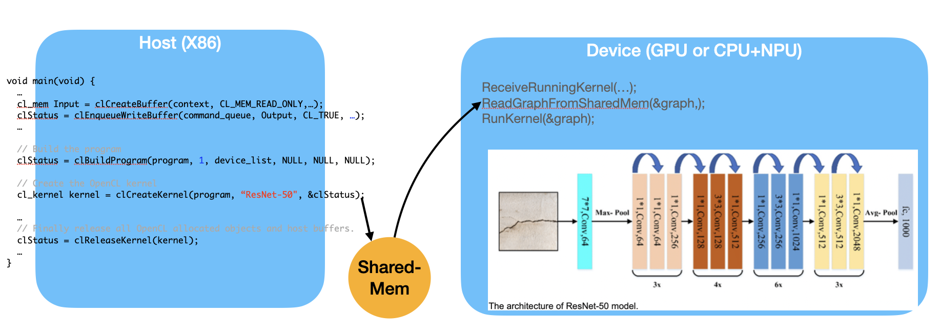
Fig. 155 Implement ML graph scheduler both on compiler and runtime
As shown in Fig. 155, the Device, such as a GPU or a CPU+NPU, is capable of running the entire ML graph. However, if the Device has only an NPU, then operations like Avg-Pool, which require CPU support, must run on the Host side. This introduces communication overhead between the Host and the Device.
Similar to OpenGL shaders, the “kernel” function may be compiled either on-line or off-line and then sent to the GPU as a programmable function.
In order to run ML (Machine Learning) efficiently, all platforms for ML on GPU/NPU implement scheduling SW both on graph compiler and runtime. If OpenCL can extend to support ML graph, then graph compiler such as TVM or Runtime from Open Source have chance to leverage the effort of scheduling SW from programmers [127]. Cuda graph is an idea like this [128] [129] .
SYCL: Using C++ templates to optimize and genertate code for OpenCL and Cuda. Provides a consistent language, APIs, and ecosystem in which to write and tune code for different accelerator architecture, CPUs, GPUs, and FPGAs [130].
SYCL uses generic programming with templates and generic lambda functions to enable higher-level application software to be cleanly coded with optimized acceleration of kernel code across an extensive range of acceleration backend APIs, such as OpenCL and CUDA [131].
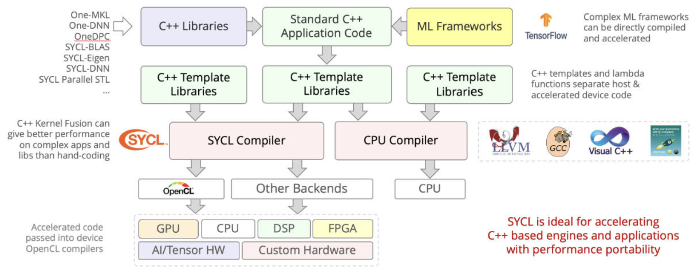
Fig. 156 SYCL = C++ template and compiler for Data Parallel Applications on AI on CPUs, GPUs and HPGAs.
DPC++ (OneDPC) compiler: Based on SYCL, DPC++ can compile the DPC++ language for both CPU host and GPU device. DPC++ (Data Parallel C++) is a language developed by Intel and may be adopted into standard C++. The GPU-side (kernel code) is written in C++ but does not support exception handling [132] [133].
Features of Kernel Code:
Not supported:
Dynamic polymorphism, dynamic memory allocations (therefore no object management using new or delete operators), static variables, function pointers, runtime type information (RTTI), and exception handling. No virtual member functions, and no variadic functions, are allowed to be called from kernel code. Recursion is not allowed within kernel code.
Supported:
Lambdas, operator overloading, templates, classes, and static polymorphism [134].